[1]:

from UFalcon import construct_maps, utils
import numpy as np
import healpy as hp
from astropy.cosmology import FlatLambdaCDM
import matplotlib.pyplot as plt
import astropy

In this notebook we demonstrate using UFalcon to produce cosmological signal maps for:¶

Galaxy weak lensing (kappa and gamma)
Galaxy clustering
CMB lensing
CMB ISW

For this we use the helper class “construct_maps” which collates the functions in the rest of the package to produce cosmological signal maps. This class can be seen as an easy starting point for an independent user.

Load in the raw lightcone shell array and the upper and lower redshift limits of each shell¶

[2]:

maps = np.load('shells_example.npz',mmap_mode="r")['maps'] #mmap_mode="r" allows us to be economical with memory usage
z_low = np.load('z_low.npy')
z_high = np.load('z_high.npy')
print(z_low)
print(z_high)

[0.         0.01277548 0.02578057 0.03902289 0.05251003 0.06625001
 0.08025129 0.09452274 0.1090737  0.1239141  0.1390541  0.1545049
 0.1702779  0.1863854  0.2028402  0.2196561  0.2368474  0.2544296
 0.2724188  0.2908324  0.3096887  0.3290072  0.3488088  0.3691156
 0.3899513  0.4113412  0.4333125  0.4558939  0.4791168  0.5030144
 0.5276226  0.5529801  0.5791287  0.6061132  0.6339825  0.6627892
 0.6925908  0.7234494  0.7554329  0.7886154  0.823078   0.8589094
 0.8962073  0.9350792  0.9756439 ]
[0.01277548 0.02578057 0.03902289 0.05251003 0.06625001 0.08025129
 0.09452274 0.1090737  0.1239141  0.1390541  0.1545049  0.1702779
 0.1863854  0.2028402  0.2196561  0.2368474  0.2544296  0.2724188
 0.2908324  0.3096887  0.3290072  0.3488088  0.3691156  0.3899513
 0.4113412  0.4333125  0.4558939  0.4791168  0.5030144  0.5276226
 0.5529801  0.5791287  0.6061132  0.6339825  0.6627892  0.6925908
 0.7234494  0.7554329  0.7886154  0.823078   0.8589094  0.8962073
 0.9350792  0.9756439  1.018033  ]

[3]:

print(f"In this example the lightcone is produced up to redshift: {z_high[-1]}")

In this example the lightcone is produced up to redshift: 1.0180330276489258

Lets plot a single lighcone shell to see what this looks like¶

[4]:

shell_no = 30
zi = z_low[shell_no]
zf = z_high[shell_no]

# Format the redshifts to three significant figures
zi_formatted = "{:.3g}".format(zi)
zf_formatted = "{:.3g}".format(zf)

hp.mollview(maps[shell_no], title=f"Lightcone shell between redshifts {zi_formatted} to {zf_formatted}", cmap='jet')

Lets set-up UFalcon¶

Firstly we can set up a helper class called “construct_maps”. This allows one to easily create probe maps and collates the funtions in the other parts of the code together in one place. For this we need to suply the simulation cosmology and some details of the simulation (boxsize, n_particles)

[5]:

#Set up cosmology of sims
eV = astropy.units.eV
Omega_m= 0.26
Omega_b = 0.0493
sigma_8 = 0.84
Neff = 3.046
H0 = 67.36
O_nu =0.001422554 #neutrino energy density
cosmo = FlatLambdaCDM(H0=H0, Om0=Omega_m-O_nu, Neff=Neff,Ob0=Omega_b, m_nu=0.02*eV, Tcmb0=2.7255)

[6]:

#Set up of simulation parameters for example
boxsize = (900 / 1000) / (H0 / 100.) # Convert 900 Mpc/h into Gpc
n_particles = 832**3

#Desired output set up
nside = 128 #output maps will have nside=128, this must be lower or equal to the input nside of the simulation lightcone maps
zi=0.0 #compute the contribution from z=0
zf=1.05 #compute the contribution to the given signal until z~1 (this is as far as our simultions allow)

[7]:

construct_class = construct_maps.construct_map_cosmogrid(maps=maps, z_low=z_low, z_high=z_high,
         nside=nside, boxsize=boxsize, cosmo=cosmo, n_particles=n_particles, zi=zi, zf=zf)

CMB weak lensing¶

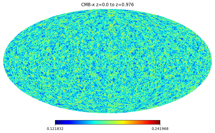
Lets start with the simplest of UFalcon maps: the map produced for CMB wek lensing. This assumes a single source at redshift z=1090 (recombination) and computes the lensing convergence kappa map for the supplied DM lightcone shells. Due to the limited redshift range of the simulation (in this case going only up to z~1) we can only compute the contribution up until this maximum redshift- one could then consider adding a gaussian realization for the high-redshift aprt of this probe.

[8]:

cmb_kappa_map = construct_class.construct_kappa_cmb_map()

actual zmax for cmb kappa: 1.018033
Processing shell 1 / 45
Processing shell 2 / 45
Processing shell 3 / 45
Processing shell 4 / 45
Processing shell 5 / 45
Processing shell 6 / 45
Processing shell 7 / 45
Processing shell 8 / 45
Processing shell 9 / 45
Processing shell 10 / 45
Processing shell 11 / 45
Processing shell 12 / 45
Processing shell 13 / 45
Processing shell 14 / 45
Processing shell 15 / 45
Processing shell 16 / 45
Processing shell 17 / 45
Processing shell 18 / 45
Processing shell 19 / 45
Processing shell 20 / 45
Processing shell 21 / 45
Processing shell 22 / 45
Processing shell 23 / 45
Processing shell 24 / 45
Processing shell 25 / 45
Processing shell 26 / 45
Processing shell 27 / 45
Processing shell 28 / 45
Processing shell 29 / 45
Processing shell 30 / 45
Processing shell 31 / 45
Processing shell 32 / 45
Processing shell 33 / 45
Processing shell 34 / 45
Processing shell 35 / 45
Processing shell 36 / 45
Processing shell 37 / 45
Processing shell 38 / 45
Processing shell 39 / 45
Processing shell 40 / 45
Processing shell 41 / 45
Processing shell 42 / 45
Processing shell 43 / 45
Processing shell 44 / 45
Processing shell 45 / 45

[9]:

hp.mollview(cmb_kappa_map, title=r"CMB-$\kappa$ z=0.0 to z=0.976", cmap='jet')

Galaxy Weak lensing¶

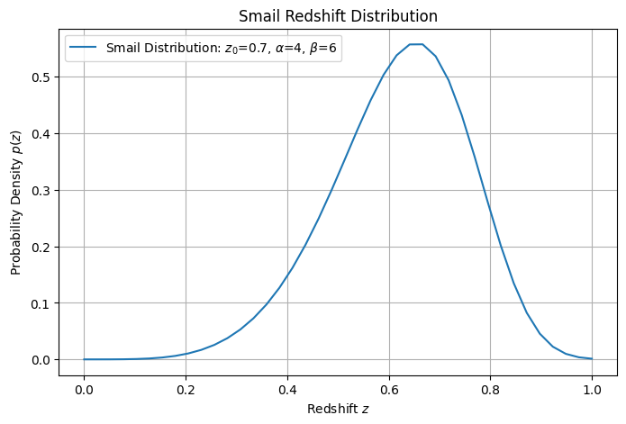
For this we need to supply a redshift distribution for the source galaxies so we begin by assuming a simple Smail distribution

[10]:

#Example photometric reshift distribution

# Define the Smail distribution
def smail(z, alpha, beta, z0):
    return (z**alpha / z0**(alpha+1)) * np.exp(-(z/z0)**beta)

# Parameters
alpha = 4
beta = 6
z0 = 0.7

num_points = 40
z = np.linspace(0, 1, num_points)
p_z = smail(z, alpha, beta, z0) #not necessary to be normalized- UFalcon takes care of this

#Put the redshift distribution in 2D-array form as required by UFalcon code
n_z = np.zeros((num_points,2))
n_z[:,0] = z
n_z[:,1] = p_z

# Plot the distribution
plt.figure(figsize=(8, 5))
plt.plot(n_z[:,0],n_z[:,1], label=f'Smail Distribution: $z_0$={z0}, $\\alpha$={alpha}, $\\beta$={beta}')
plt.xlabel('Redshift $z$')
plt.ylabel('Probability Density $p(z)$')
plt.title('Smail Redshift Distribution')
plt.legend()
plt.grid(True)
plt.show()

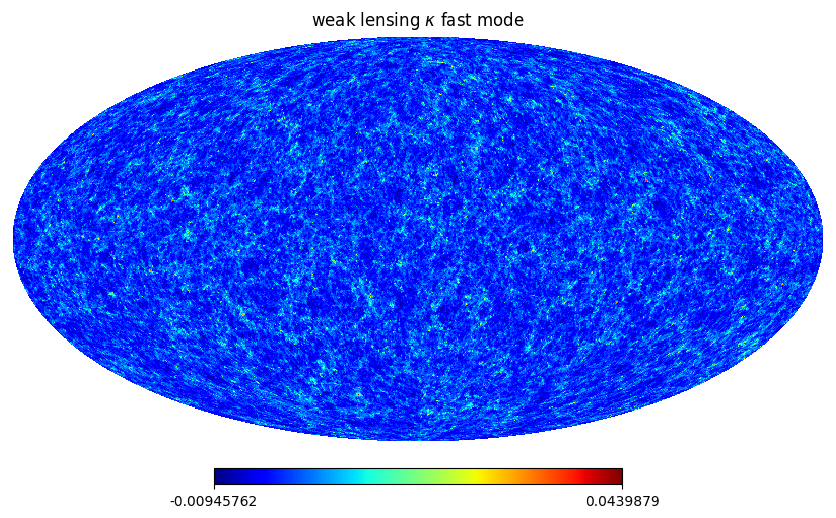
UFalcon also includes the option of applying a shift to the photometric redshift distribution and can compute the IA signal using the NLA model

[11]:

IA = 0.0 #no instrinsic alignment in this example
shift_nz = 0.0  #no delta z shift

[31]:

#NB if IA is non-zero here the produced map will contain a cosmological signal + an IA signal
#UFalcon also allows for a computation of the IA signal alone (see later)

#In this example we use "fast_mode" this should always be tested against the more robust default (fast_mode=False)- see comparison later
kappa_wl_map_fast_mode = construct_class.construct_kappa_map(n_of_z=n_z, shift_nz=shift_nz, IA=IA, fast_mode=True, \
            fast_mode_num_points_1d=13, fast_mode_num_points_2d=512)

PURE COSMOLOGICAL SIGNAL WITH NO IA BEING COMPUTED
Processing shell 1 / 45
Processing shell 2 / 45
Processing shell 3 / 45
Processing shell 4 / 45
Processing shell 5 / 45
Processing shell 6 / 45
Processing shell 7 / 45
Processing shell 8 / 45
Processing shell 9 / 45
Processing shell 10 / 45
Processing shell 11 / 45
Processing shell 12 / 45
Processing shell 13 / 45
Processing shell 14 / 45
Processing shell 15 / 45
Processing shell 16 / 45
Processing shell 17 / 45
Processing shell 18 / 45
Processing shell 19 / 45
Processing shell 20 / 45
Processing shell 21 / 45
Processing shell 22 / 45
Processing shell 23 / 45
Processing shell 24 / 45
Processing shell 25 / 45
Processing shell 26 / 45
Processing shell 27 / 45
Processing shell 28 / 45
Processing shell 29 / 45
Processing shell 30 / 45
Processing shell 31 / 45
Processing shell 32 / 45
Processing shell 33 / 45
Processing shell 34 / 45
Processing shell 35 / 45
Processing shell 36 / 45
Processing shell 37 / 45
Processing shell 38 / 45
Processing shell 39 / 45
Processing shell 40 / 45
Processing shell 41 / 45
Processing shell 42 / 45
Processing shell 43 / 45
Processing shell 44 / 45
Processing shell 45 / 45

[13]:

hp.mollview(kappa_wl_map_fast_mode, title=r"weak lensing $\kappa$ fast mode", cmap='jet')

[14]:

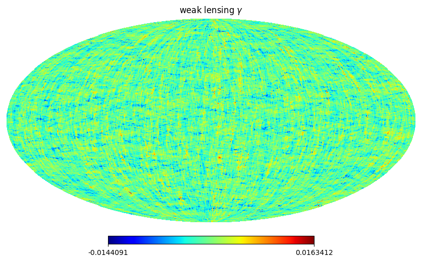
#UFalcon also provides a convenient function to switch between weak lensing kappa and weak lensing gamma maps using the Kaiser-Squires transform
#(see equations 24/25 in https://arxiv.org/abs/1703.09233)

#Use pixelweights for the map2alm transformation: This delivers the most accurate transform according to healpy, but requires
#the pixel weights, which will be downloaded automatically.

gam1, gam2 = utils.kappa_to_gamma(
            kappa_wl_map_fast_mode, use_pixel_weights=True)

/Users/alexreeves/Documents/local_software/UFalcon/src/UFalcon/utils.py:192: RuntimeWarning: divide by zero encountered in divide
  -np.sqrt(((ell + 2.0) * (ell - 1)) / ((ell + 1) * ell)),
/Users/alexreeves/Documents/local_software/UFalcon/src/UFalcon/utils.py:192: RuntimeWarning: invalid value encountered in sqrt
  -np.sqrt(((ell + 2.0) * (ell - 1)) / ((ell + 1) * ell)),

[15]:

hp.mollview(gam1, title=r"weak lensing $\gamma$", cmap='jet')

[16]:

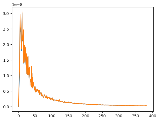
#Check that the power spectra match up as expected
cl_gamma = hp.anafast([np.zeros_like(gam1), gam1, gam2])[1]
cl_kappa = hp.anafast(kappa_wl_map_fast_mode)
plt.plot(cl_gamma)
plt.plot(cl_kappa)

[16]:

[<matplotlib.lines.Line2D at 0x15416ea50>]

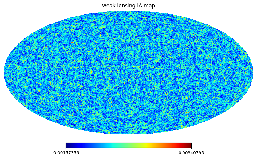
Finally UFalcon also allows to compute the IA contribution alone

[17]:

kappa_IA = construct_class.construct_IA_map(n_of_z=n_z, shift_nz=shift_nz, IA=1.0)

Processing shell 1 / 45
min() arg is an empty sequence
Processing shell 2 / 45
Processing shell 3 / 45
min() arg is an empty sequence
Processing shell 4 / 45
Processing shell 5 / 45
min() arg is an empty sequence
Processing shell 6 / 45
Processing shell 7 / 45
min() arg is an empty sequence
Processing shell 8 / 45
Processing shell 9 / 45
min() arg is an empty sequence
Processing shell 10 / 45
Processing shell 11 / 45
Processing shell 12 / 45
min() arg is an empty sequence
Processing shell 13 / 45
Processing shell 14 / 45
min() arg is an empty sequence
Processing shell 15 / 45
Processing shell 16 / 45
Processing shell 17 / 45
min() arg is an empty sequence
Processing shell 18 / 45
Processing shell 19 / 45
Processing shell 20 / 45
Processing shell 21 / 45
min() arg is an empty sequence
Processing shell 22 / 45
Processing shell 23 / 45
Processing shell 24 / 45
Processing shell 25 / 45
Processing shell 26 / 45
min() arg is an empty sequence
Processing shell 27 / 45
Processing shell 28 / 45
Processing shell 29 / 45
Processing shell 30 / 45
Processing shell 31 / 45
Processing shell 32 / 45
Processing shell 33 / 45
Processing shell 34 / 45
Processing shell 35 / 45
Processing shell 36 / 45
Processing shell 37 / 45
Processing shell 38 / 45
Processing shell 39 / 45
Processing shell 40 / 45
Processing shell 41 / 45
Processing shell 42 / 45
Processing shell 43 / 45
Processing shell 44 / 45
Processing shell 45 / 45
min() arg is an empty sequence

[18]:

hp.mollview(kappa_IA, title=r"weak lensing IA map", cmap='jet')

Galaxy clustering¶

Here we use the same example Smail redshift distribution as for the weak lensing probe, now this represents the redshift distribution of the galaxy survey we are modeling

[19]:

lin_bias = 1.5 #The galaxy linear bias (more complex bias modelas are under development)

galaxy_delta = construct_class.construct_delta_map(n_of_z=n_z, lin_bias=lin_bias)

Processing shell 1 / 45
Processing shell 2 / 45
Processing shell 3 / 45
Processing shell 4 / 45
Processing shell 5 / 45
Processing shell 6 / 45
Processing shell 7 / 45
Processing shell 8 / 45
Processing shell 9 / 45
Processing shell 10 / 45
Processing shell 11 / 45
Processing shell 12 / 45
Processing shell 13 / 45
Processing shell 14 / 45
Processing shell 15 / 45
Processing shell 16 / 45
Processing shell 17 / 45
Processing shell 18 / 45
Processing shell 19 / 45
Processing shell 20 / 45
Processing shell 21 / 45
Processing shell 22 / 45
Processing shell 23 / 45
Processing shell 24 / 45
Processing shell 25 / 45
Processing shell 26 / 45
Processing shell 27 / 45
Processing shell 28 / 45
Processing shell 29 / 45
Processing shell 30 / 45
Processing shell 31 / 45
Processing shell 32 / 45
Processing shell 33 / 45
Processing shell 34 / 45
Processing shell 35 / 45
Processing shell 36 / 45
Processing shell 37 / 45
Processing shell 38 / 45
Processing shell 39 / 45
Processing shell 40 / 45
Processing shell 41 / 45
Processing shell 42 / 45
Processing shell 43 / 45
Processing shell 44 / 45
Processing shell 45 / 45

[20]:

hp.mollview(galaxy_delta, title=r"$\delta_g$ map", cmap='jet')

ISW probe¶

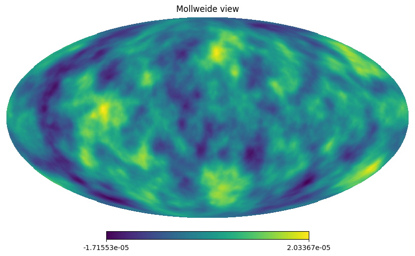
Finally, lets how an example of the (currently experimental) ISW probe. This implementation is based off of that presented in https://arxiv.org/abs/2103.14654.

[21]:

# To minimize unphysical features due to box replications, we recommend setting zmax to None.
# This allows the pipeline to determine a recommended zmax value that reduces such features in the final maps.
isw_map = construct_class.construct_isw_map(zmax_for_box=None)

Creating SBT class. This may take a few seconds...
zmax_for_box = None was passed. Using the recommended value of 0.50 computed based on the boxsize 900.00 Mpc/h.
Warning: no alpha function provided, so the default is being used. However, this default has only been tested on a Cosmogrid set up, so proceed with caution.
converting to alm shell 1 / 45
converting to alm shell 2 / 45
converting to alm shell 3 / 45
converting to alm shell 4 / 45
converting to alm shell 5 / 45
converting to alm shell 6 / 45
converting to alm shell 7 / 45
converting to alm shell 8 / 45
converting to alm shell 9 / 45
converting to alm shell 10 / 45
converting to alm shell 11 / 45
converting to alm shell 12 / 45
converting to alm shell 13 / 45
converting to alm shell 14 / 45
converting to alm shell 15 / 45
converting to alm shell 16 / 45
converting to alm shell 17 / 45
converting to alm shell 18 / 45
converting to alm shell 19 / 45
converting to alm shell 20 / 45
converting to alm shell 21 / 45
converting to alm shell 22 / 45
converting to alm shell 23 / 45
converting to alm shell 24 / 45
converting to alm shell 25 / 45
converting to alm shell 26 / 45
converting to alm shell 27 / 45
converting to alm shell 28 / 45
converting to alm shell 29 / 45
converting to alm shell 30 / 45
converting to alm shell 31 / 45
Slice not in zmin and zmax range.
converting to alm shell 32 / 45
Slice not in zmin and zmax range.
converting to alm shell 33 / 45
Slice not in zmin and zmax range.
converting to alm shell 34 / 45
Slice not in zmin and zmax range.
converting to alm shell 35 / 45
Slice not in zmin and zmax range.
converting to alm shell 36 / 45
Slice not in zmin and zmax range.
converting to alm shell 37 / 45
Slice not in zmin and zmax range.
converting to alm shell 38 / 45
Slice not in zmin and zmax range.
converting to alm shell 39 / 45
Slice not in zmin and zmax range.
converting to alm shell 40 / 45
Slice not in zmin and zmax range.
converting to alm shell 41 / 45
Slice not in zmin and zmax range.
converting to alm shell 42 / 45
Slice not in zmin and zmax range.
converting to alm shell 43 / 45
Slice not in zmin and zmax range.
converting to alm shell 44 / 45
Slice not in zmin and zmax range.
converting to alm shell 45 / 45
Slice not in zmin and zmax range.
Converting to sbt...
Finding zeros for Bessel function up to n = 129
Constructing l and n value grid
Pre-compute spherical Bessel integrals
Computing spherical Bessel Transform from spherical harmonics
mean redshift of slice 1 / 30: 0.01
mean redshift of slice 2 / 30: 0.02
mean redshift of slice 3 / 30: 0.03
mean redshift of slice 4 / 30: 0.05
mean redshift of slice 5 / 30: 0.06
mean redshift of slice 6 / 30: 0.07
mean redshift of slice 7 / 30: 0.09
mean redshift of slice 8 / 30: 0.10
mean redshift of slice 9 / 30: 0.12
mean redshift of slice 10 / 30: 0.13
mean redshift of slice 11 / 30: 0.15
mean redshift of slice 12 / 30: 0.16
mean redshift of slice 13 / 30: 0.18
mean redshift of slice 14 / 30: 0.19
mean redshift of slice 15 / 30: 0.21
mean redshift of slice 16 / 30: 0.23
mean redshift of slice 17 / 30: 0.25
mean redshift of slice 18 / 30: 0.26
mean redshift of slice 19 / 30: 0.28
mean redshift of slice 20 / 30: 0.30
mean redshift of slice 21 / 30: 0.32
mean redshift of slice 22 / 30: 0.34
mean redshift of slice 23 / 30: 0.36
mean redshift of slice 24 / 30: 0.38
mean redshift of slice 25 / 30: 0.40
mean redshift of slice 26 / 30: 0.42
mean redshift of slice 27 / 30: 0.44
mean redshift of slice 28 / 30: 0.47
mean redshift of slice 29 / 30: 0.49
mean redshift of slice 30 / 30: 0.52

[22]:

isw_map

[22]:

array([-2.94393808e-06, -3.15297772e-06, -3.58408665e-06, ...,
       -7.79299515e-07, -1.37734206e-06, -1.36757380e-06])

[23]:

hp.mollview(isw_map)

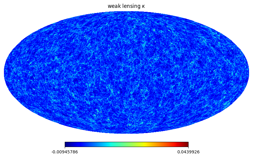
Finally, lets see how good the approximation of “fast mode” is for the kappa WL.¶

This will take ~10 minutes to run on a laptop

[24]:

kappa_wl_map = construct_class.construct_kappa_map(n_of_z=n_z, shift_nz=shift_nz, IA=IA, fast_mode=False) #no fast mode

PURE COSMOLOGICAL SIGNAL WITH NO IA BEING COMPUTED
Processing shell 1 / 45
Processing shell 2 / 45
Processing shell 3 / 45
Processing shell 4 / 45
Processing shell 5 / 45
Processing shell 6 / 45
Processing shell 7 / 45
Processing shell 8 / 45
Processing shell 9 / 45
Processing shell 10 / 45
Processing shell 11 / 45
Processing shell 12 / 45
Processing shell 13 / 45
Processing shell 14 / 45
Processing shell 15 / 45
Processing shell 16 / 45
Processing shell 17 / 45
Processing shell 18 / 45
Processing shell 19 / 45
Processing shell 20 / 45
Processing shell 21 / 45
Processing shell 22 / 45
Processing shell 23 / 45
Processing shell 24 / 45
Processing shell 25 / 45
Processing shell 26 / 45
Processing shell 27 / 45
Processing shell 28 / 45
Processing shell 29 / 45
Processing shell 30 / 45
Processing shell 31 / 45
Processing shell 32 / 45
Processing shell 33 / 45
Processing shell 34 / 45
Processing shell 35 / 45
Processing shell 36 / 45
Processing shell 37 / 45
Processing shell 38 / 45
Processing shell 39 / 45
Processing shell 40 / 45
Processing shell 41 / 45
Processing shell 42 / 45
Processing shell 43 / 45
Processing shell 44 / 45
Processing shell 45 / 45

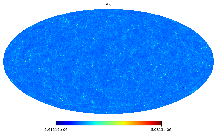
[28]:

hp.mollview(kappa_wl_map, title=r"weak lensing $\kappa$", cmap='jet')
hp.mollview(kappa_wl_map_fast_mode, title=r"weak lensing $\kappa$ fast mode", cmap='jet')

[29]:

hp.mollview(kappa_wl_map-kappa_wl_map_fast_mode, title=r"$\Delta \kappa$", cmap='jet')

[ ]: