Usage¶

Background¶

• Angular diameter distance at a = 0.4:

  >>> cosmo.background.dist_ang_a(a=0.4)
  array([ 1762.38876138])
  

• Luminosity distance at a = 0.6 and 0.8

  >>> cosmo.background.dist_lum_a(a=[0.6,0.8])
  array([ 4048.4298942 ,  1266.53970396])
  

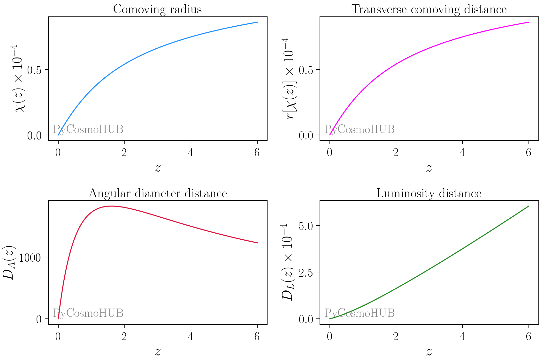
• Cosmological distances as a function of a:

  >>> cosmo.background.dist_rad_a(a)      # comoving radius
  >>> cosmo.background.dist_trans_a(a)    # transverse comoving distance
  >>> cosmo.background.dist_ang_a(a)      # angular diameter distance
  >>> cosmo.background.dist_lum_a(a)      # luminosity distance
  

Image created with the PyCosmoHUB.

Linear and non-linear perturbations¶

• Growth factor at a = 0.5 and 1.0:

  >>> cosmo.lin_pert.growth_a(a=[.5,1.])
  array([ 0.61200153,  1.])
  

• Linear and non linear matter power spectrum at a = 1 for a grid of k values:

  >>> import numpy as np
  >>> pk_l = cosmo.lin_pert.powerspec_a_k(a=1., k=np.logspace(-3,0))
  >>> pk_nl = cosmo.nonlin_pert.powerspec_a_k(a=1., k=np.logspace(-3,0))
  

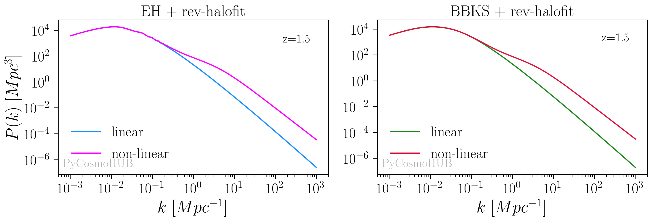
• Linear and non linear matter power spectrum as a function of k, at redshift z=1.5. Examples are given using both Eisenstein & Hu and BBKS linear fitting functions, and the revised version of Halofit for the non-linear fitting function:

  >>> # Set the non-linear fitting function
  >>> cosmo.set(pk_nonlin_type = 'rev_halofit')
  

  >>> # Set the linear fitting function to EH
  >>> cosmo.set(pk_type = 'EH')
  >>> # Compute the linear and non-linear power spectra with rev_halofit+EH
  >>> pk_lin_EH = cosmo.lin_pert.powerspec_a_k(1./(1+z), k)[:,0]
  >>> pk_nonlin_EH = cosmo.nonlin_pert.powerspec_a_k(1./(1+z), k)[:,0]
  

  >>> # Set the linear fitting function to BBKS
  >>> cosmo.set(pk_type = 'BBKS')
  >>> # # Compute the linear and non-linear power spectra with rev_halofit+BBKS
  >>> pk_lin_BBKS = cosmo.lin_pert.powerspec_a_k(1./(1+z), k)[:,0]
  >>> pk_nonlin_BBKS = cosmo.nonlin_pert.powerspec_a_k(1./(1+z), k)[:,0]
  

Image created with the PyCosmoHUB.

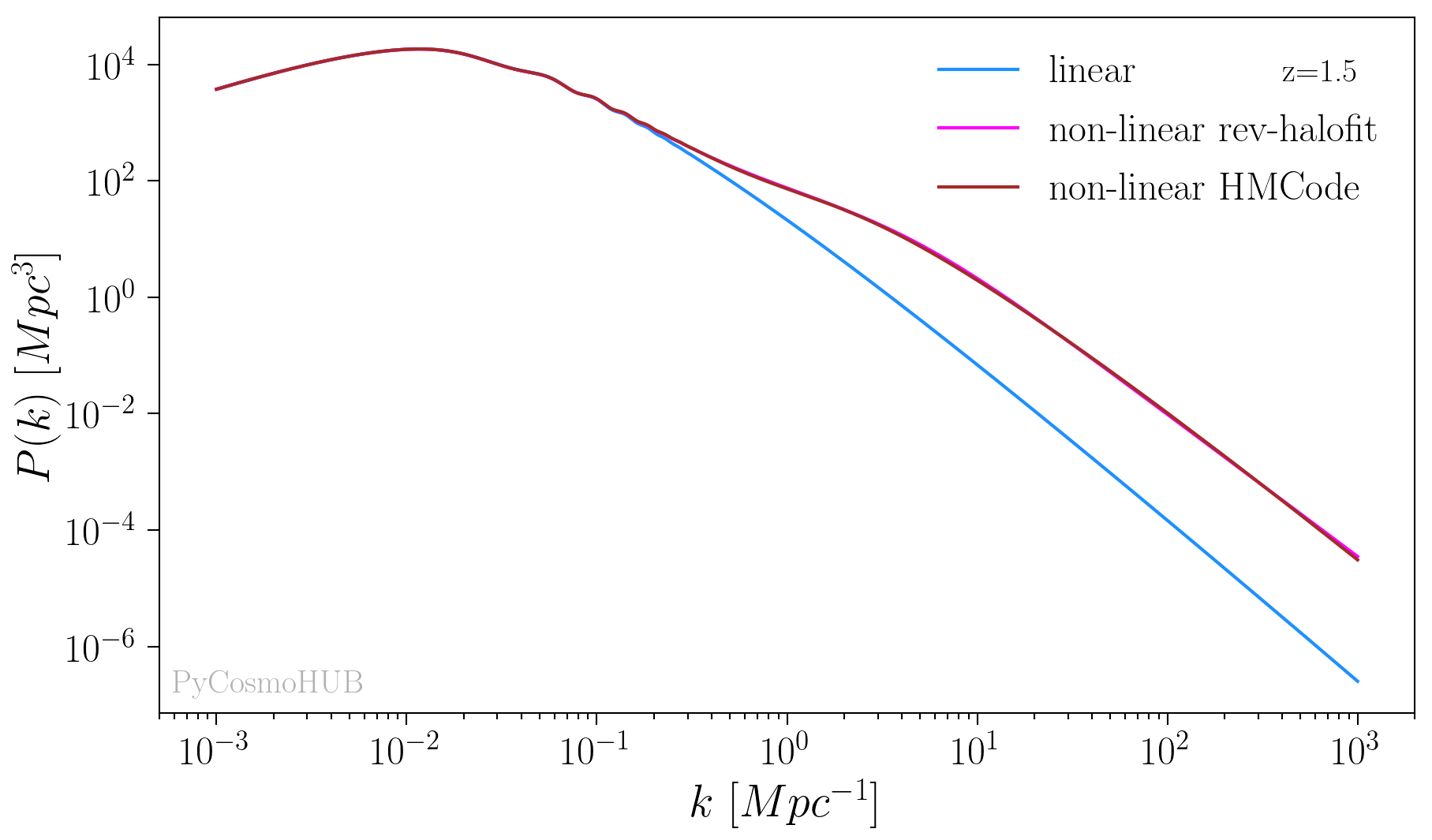
• Non linear matter power spectrum computed with the Mead et al. model, at redshift z=1.5:

  >>> cosmo.set(pk_type='EH', pk_nonlin_type='mead')
  >>> pk_nonlin_hmcode = cosmo.nonlin_pert.powerspec_a_k(1./(1+z), k)[:,0]
  

Image created with the PyCosmoHUB.

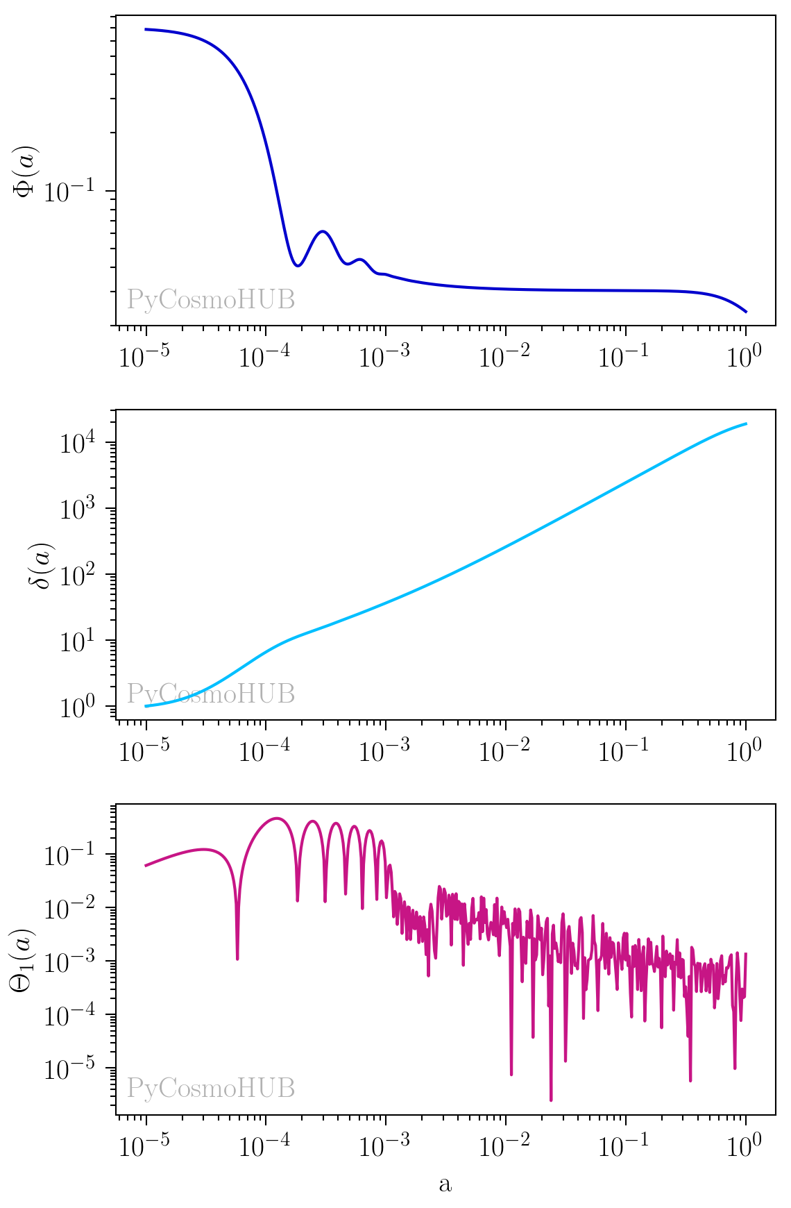
Perturbations with the Boltzmann solver¶

• Linear perturbations can also be computed using the Boltzmann solver. In order to use the Boltzmann solver, set pk_type=”boltz”. It is also recommended to use pk_norm_type=”A_s” with the Boltzmann solver. We show an example of the computation of the fields for a specific k value (k=0.2 \(h^{-1}\mathrm{Mpc}\)) as a function of the scale factor a:

  >>> cosmo = PyCosmo.build("lcdm")
  >>> cosmo.set(pk_type='boltz', pk_norm_type='A_s', pk_norm=2.1e-9)
  >>> fields = cosmo.lin_per.fields(k=0.2, grid=np.log(np.logspace(-5,0,500)))
  >>> fields.Phi, fields.delta, fields.Theta[1]
  

Image created with the PyCosmoHUB.

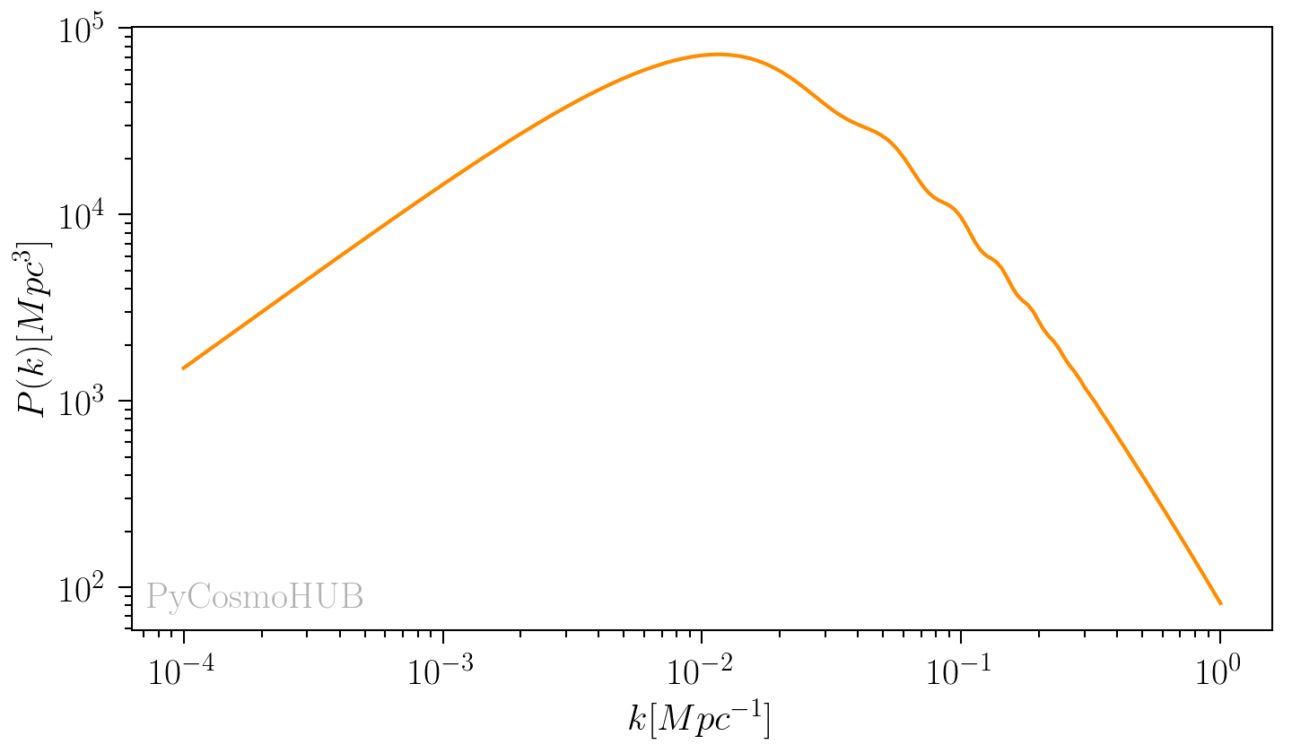
• The total matter power spectrum is computed using the powerspec_a_k function, equivalently to the example of the fitting functions:

  >>> pk_boltz = cosmo.lin_pert.powerspec_a_k(a=1., k)[:,0]
  

Image created with the PyCosmoHUB.

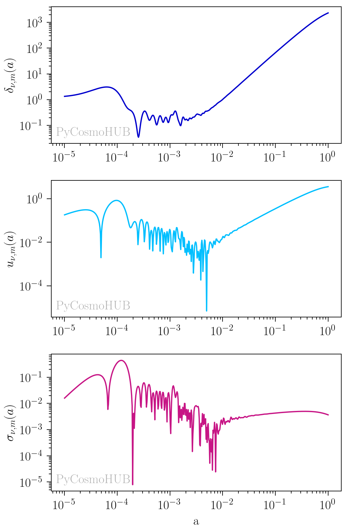
Massive neutrinos¶

• We show an example of the linear perturbation computation for a massive neutrino model. We first set A_s normalization, increase the total mass of the neutrinos (while keeping the number to 3) and use the RSA to speed up the computation.

  >>> cosmo_nu = PyCosmo.build("mnulcdm", rsa=True)
  >>> cosmo_nu.set(pk_type='boltz', pk_norm_type='A_s', pk_norm=2.1e-9, massive_nu_total_mass=0.5)
  >>> fields_nu = cosmo_nu.lin_pert.fields(k=0.2, grid = np.log(np.logspace(-5,0,500)))
  

• We now plot the massive neutrino fields: fields_nu.delta_nu_m, fields_nu.u_nu_m and fields_nu.sigma_nu_m

Image created with the PyCosmoHUB.

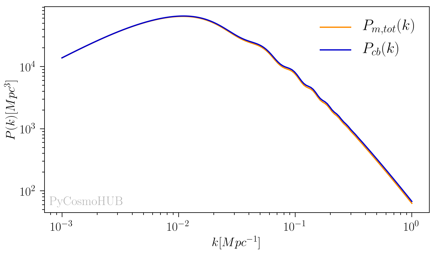
• We compute the total matter power spectrum and the cold dark matter and baryon power spectrum and look at the difference:

  >>> ps_nu = cosmo_nu.lin_pert.powerspec_a_k(k=kvec, a=1.)
  >>> ps_nu_cb = cosmo_nu.lin_pert.powerspec_cb_a_k(k=kvec, a=1.)
  

Image created with the PyCosmoHUB.

Observables¶

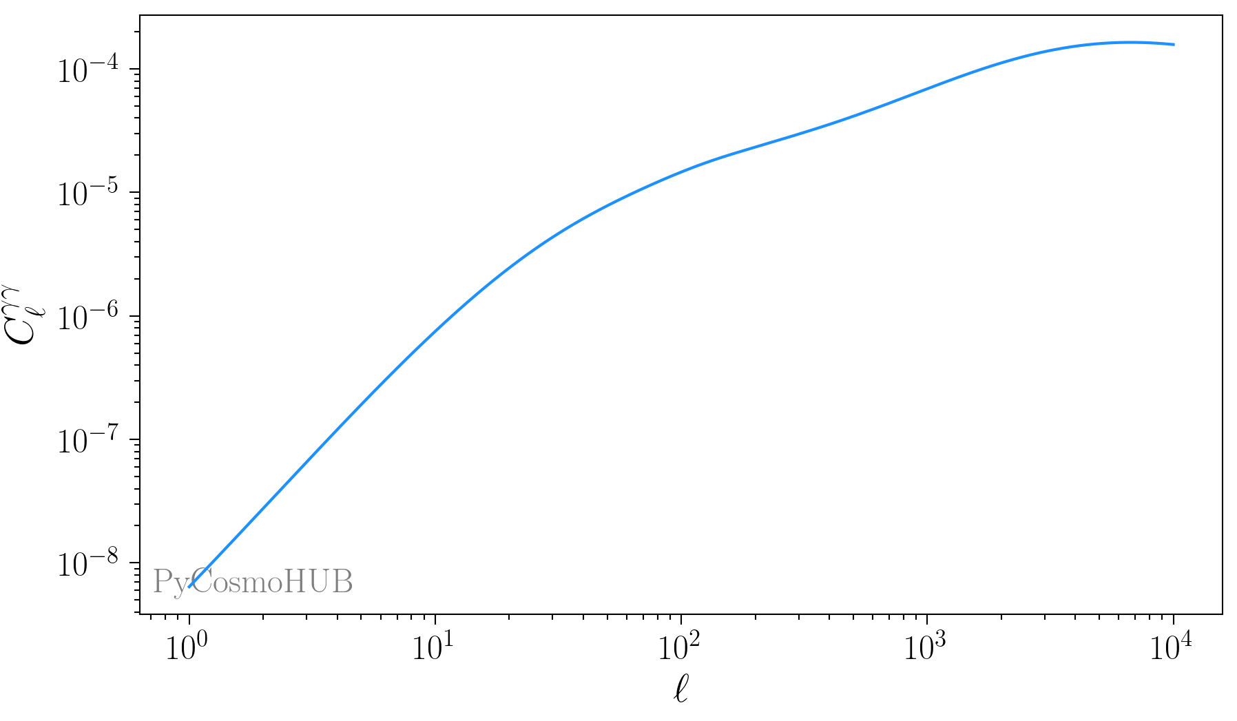
• Computation of the weak lensing power spectrum \(C_{\ell}^{\gamma \gamma}\) using non-linear perturbations:

  >>> # PyCosmo instance
  >>> cosmo = PyCosmo.Cosmo()
  

  >>> # Set the fitting functions for the power spectrum
  >>> cosmo.set(pk_type='EH', pk_nonlin_type='rev_halofit')
  >>> # Note: 'perturb': 'nonlinear' can be replaced with 'linear' by the user.
  >>> clparams = {'nz': ['smail', 'smail'],
  >>>             'z0': 1.13,
  >>>             'beta': 2.,
  >>>             'alpha': 2.,
  >>>             'probes': ['gamma', 'gamma'],
  >>>             'perturb': 'nonlinear',
  >>>             'normalised': False,
  >>>             'bias': 1.,
  >>>             'm': 0,
  >>>             'z_grid': np.array([0.0001, 5., 1000])
  >>>             }
  >>> obs = PyCosmo.Obs()
  >>> cls_haloEH = obs.cl(ells, cosmo, clparams)
  

Image created with PyCosmoHUB.