Generating Beam Models with SERVAL
This notebook demonstrates several SERVAL workflows for constructing and storing beam models that can be used by the CLI. We start with analytic beam patterns, but also show how e.g. CST simulated beams or arbitary callables can be used.
- Analytic voltage beams —
from_gaussianandfrom_airycreateTIRSVoltageBeamobjects from parameterised models, which we then rotate to the pointed basis, normalise, and save to Zarr. - Beam families with pointing offsets — generate per-dish voltage beams with
random pointing errors using
offset_pointing. - CST farfield imports —
from_cst_farfieldsreads CST farfield exports and builds interpolatedTIRSVoltageBeamobjects. - Power-beam construction from voltage beams — derive
TIRSPowerBeamproducts from pairs of voltage beams. - Direct analytic and callable power beams — build simplified scalar power
beams with
from_gaussian,from_airy, orfrom_scalar_callable.
import tempfile
from pathlib import Path
import warnings

import numpy as np
import matplotlib as mpl
import matplotlib.pyplot as plt

import astropy.coordinates as coords
from astropy import units

from serval.containers import TIRSVoltageBeam, TIRSPowerBeam, CSTBeamInterpolator
from serval.rotate import offset_pointing
from serval.sht import grid_template
from serval.helpers import grid_theta_phi
from serval.utils import airy_pattern, gaussian_pattern

plt.style.use("./example_style.mplstyle")
mpl.rcParams["text.usetex"] = False
# For clean notebook output
warnings.filterwarnings("ignore")
_ = np.seterr(divide="ignore")
latitude = coords.Latitude("-30d41m47.0s").rad
longitude = coords.Longitude("21d34m20.0s").rad

# Nominal pointing: zenith
nominal_alt = np.pi / 2
nominal_az = np.pi
nominal_bs = 0.0

# Use a small frequency subset
frequencies_MHz = np.linspace(400, 800, 5)

# Harmonic bandlimits
voltage_beam_lmax = 200
pointed_mmax = 50
1. Analytic beam models
SERVAL provides two built-in voltage beam constructors based on analytic models for
use in testing/simple simulations. Both model the co-polarisation voltage response;
the cross-polarisation level is set separately via cross_pol_factor.
-
from_gaussian— a Gaussian voltage pattern. Supports optional elliptical asymmetry (asymmetry_ratio,asymmetry_angle) and cross-polarisation (cross_pol_factor). -
from_airy— an Airy disk pattern \(2 J_1(x)/x\), the far-field diffraction pattern of a uniformly-illuminated circular aperture. Same asymmetry and cross-pol options.
Both models are calibrated so that the power-beam FWHM equals approximately
\(1.029\,\lambda / D_\mathrm{eff}\) — the exact FWHM of the Airy disk for a
uniformly-illuminated aperture. This means the Gaussian and Airy constructors produce
beams with the same FWHM for a given D_eff, making them easy to compare.
Note: For more realistic beams, see the constructors that follow which take CST outputs or consider defining callable beam models that can be used with
TIRSVoltageBeam.from_ludwig3orTIRSVoltageBeam.from_thetaphi.
Both return a TIRSVoltageBeam in the TIRS frame. A typical workflow is:
construct with horizon taper -> to_pointed_basis (rotate SHT basis to the pointing frame for compact
m-mode representation) -> normalise. Although the order of the rotation and normalisation shouldn't matter.
D_eff = 6.0  # metres

common_kwargs = dict(
    D_eff=D_eff,
    lmax=voltage_beam_lmax,
    frequencies_MHz=frequencies_MHz,
    latitude=latitude,
    longitude=longitude,
    apply_horizon=True,
    cross_pol_factor=1e-3,
    horizon_taper_kwargs={"taper_width": np.radians(5)},
)

# Build TIRS-basis beams (full mmax = lmax, suitable for plotting)
vbeam_gauss_x_tirs = TIRSVoltageBeam.from_gaussian(
    polarisation="X", **common_kwargs
).normalise("power_integral")
vbeam_gauss_y_tirs = TIRSVoltageBeam.from_gaussian(
    polarisation="Y", **common_kwargs
).normalise("power_integral")
vbeam_airy_x_tirs = TIRSVoltageBeam.from_airy(
    polarisation="X", **common_kwargs
).normalise("power_integral")
vbeam_airy_y_tirs = TIRSVoltageBeam.from_airy(
    polarisation="Y", **common_kwargs
).normalise("power_integral")

print(f"Gaussian Y-pol TIRS alm shape: {vbeam_gauss_y_tirs.alm.shape}")
print(f"Airy Y-pol TIRS alm shape:     {vbeam_airy_y_tirs.alm.shape}")
Gaussian Y-pol TIRS alm shape: (2, 5, 201, 401)
Airy Y-pol TIRS alm shape:     (2, 5, 201, 401)
grid = grid_template(voltage_beam_lmax)
theta, phi = grid_theta_phi(grid, meshgrid=True)

fig, axes = plt.subplots(1, 2, figsize=(13, 5), sharey=True)
for ax, beam, label in zip(
    axes, [vbeam_gauss_y_tirs, vbeam_airy_y_tirs], ["Gaussian", "Airy"]
):
    beam_map = np.abs(beam.as_grid(pol_inds=0, freq_inds=0)**2 + beam.as_grid(pol_inds=1, freq_inds=0)**2)**0.5
    beam_dB = 20 * np.log10(beam_map)
    im = ax.pcolormesh(np.degrees(phi), np.degrees(theta), beam_dB, vmin=-60)
    ax.set_title(
        f"{label}, Y-pol\n {frequencies_MHz[0]:.0f} MHz"
    )
    ax.set_xlabel("$\phi$ [deg]")
    ax.set_xlim(0, 360)
    ax.set_ylim(180, 0)
    ax.set_aspect(1)

axes[0].set_ylabel(r"$\theta$ [deg]")
fig.colorbar(im, ax=axes, label="|E| [dB]", shrink=0.8)
plt.show()

Rotating to the pointed basis
SERVAL allows for more efficient use and storage of beam models by representing them in pointing aligned (as opposed to TIRS pole aligned) spherical harmonic decompositions. This allows for the typically azimuthally symmetric beams of certain classes of radio telescopes to be represented up to a user defined mmax. Resulting storage and computations can make use of this compactness.
Note The polarisation basis for these beams remains in the TIRS coordinate system (TIRS \(\theta\)-\(\phi\)). Only the spherical harmonic decomposition is done in a pointing oriented basis.
pointed_kwargs = dict(
    latitude=latitude,
    longitude=longitude,
    altitude=nominal_alt,
    azimuth=nominal_az,
    boresight=nominal_bs,
    mmax=pointed_mmax,
)

vbeam_gauss_x = vbeam_gauss_x_tirs.to_pointed_basis(**pointed_kwargs).normalise(
    "power_integral"
)
vbeam_gauss_y = vbeam_gauss_y_tirs.to_pointed_basis(**pointed_kwargs).normalise(
    "power_integral"
)
vbeam_airy_x = vbeam_airy_x_tirs.to_pointed_basis(**pointed_kwargs).normalise(
    "power_integral"
)
vbeam_airy_y = vbeam_airy_y_tirs.to_pointed_basis(**pointed_kwargs).normalise(
    "power_integral"
)

print(
    f"Gaussian Y-pol pointed alm shape: {vbeam_gauss_y.alm.shape}  (mmax={vbeam_gauss_y.mmax})"
)
print(
    f"Airy Y-pol pointed alm shape:     {vbeam_airy_y.alm.shape}  (mmax={vbeam_airy_y.mmax})"
)
Gaussian Y-pol pointed alm shape: (2, 5, 201, 101)  (mmax=50)
Airy Y-pol pointed alm shape:     (2, 5, 201, 101)  (mmax=50)
# Plot the beams in the pointed frame.
# as_grid requires mmax == lmax, so zero-pad the truncated pointed-basis beams.
grid_p = grid_template(voltage_beam_lmax)
theta_p, phi_p = grid_theta_phi(grid_p, meshgrid=True)

fig, axes = plt.subplots(1, 2, figsize=(13, 5), sharey=True)
for ax, beam, label in zip(
    axes,
    [vbeam_gauss_y, vbeam_airy_y],
    ["Gaussian", "Airy"],
):
    full_mmax = beam.bandlimited_to(lmax=beam.lmax, mmax=beam.lmax)
    beam_map = np.abs(full_mmax.as_grid(pol_inds=0, freq_inds=0)**2 + full_mmax.as_grid(pol_inds=1, freq_inds=0)**2)**0.5
    beam_dB = 20 * np.log10(beam_map)
    im = ax.pcolormesh(np.degrees(phi_p), np.degrees(theta_p), beam_dB, vmin=-60)
    ax.set_title(
        f"{label}, Y-pol\n {frequencies_MHz[0]:.0f} MHz"
    )
    ax.set_xlabel("$\phi$ [deg]")
    ax.set_xlim(0, 360)
    ax.set_ylim(180, 0)
    ax.set_aspect(1.0)

axes[0].set_ylabel(r"$\theta$ [deg]")
fig.colorbar(im, ax=axes, label="|E| [dB]", shrink=0.8)
fig.suptitle("Beams in the pointed frame (SHT basis = Pointing)", y=0.87)
plt.show()

Saving voltage beams to Zarr
Voltage beams can be saved to Zarr stores for later use with the SERVAL CLI
(serval gencache, serval genvis). Each beam is stored in its own group,
identified by a group_path string. The store can hold beams from different
dishes, polarisations, or beam models.
zarr_dir = tempfile.mkdtemp(prefix="serval_example_")
analytic_zarr_path = str(Path(zarr_dir) / "analytic_voltage_beams.zarr")

# Save both polarisations for each beam model
for beam, label in [
    (vbeam_gauss_x, "gaussian_X"),
    (vbeam_gauss_y, "gaussian_Y"),
    (vbeam_airy_x, "airy_X"),
    (vbeam_airy_y, "airy_Y"),
]:
    beam.to_zarr_store(
        store_location=analytic_zarr_path,
        group_path=label,
    )

print(f"Saved voltage beams to Zarr store.")

# Verify by loading one back
loaded = TIRSVoltageBeam.from_zarr_store(analytic_zarr_path, group_path="gaussian_Y")
print(
    f"Loaded back: polarisation={loaded.polarisation}, "
    f"sht_basis={loaded.sht_basis}, alm shape={loaded.alm.shape}"
)
Saved voltage beams to Zarr store.
Loaded back: polarisation=Y, sht_basis=Pointing, alm shape=(2, 5, 201, 101)
2. Beam families with pointing offsets
In a real array, each dish could have a slightly different pointing due to mechanical
tolerances. offset_pointing converts a (magnitude, direction, boresight roll)
offset into absolute (alt, az, boresight) parameters.
Below we generate a small family of Gaussian voltage beams for mispointed dishes,
saving each polarisation to a Zarr store. This is representative of the kind of
input one might use to explore mispointing systematics with serval genvis.
n_dishes = 4

rng = np.random.default_rng(1234)
offset_magnitudes = rng.standard_normal(n_dishes) * (10 * units.arcmin).to("rad").value
offset_directions = rng.uniform(0, high=2 * np.pi, size=n_dishes)
offset_boresights = rng.standard_normal(n_dishes) * (5 * units.arcmin).to("rad").value

family_zarr_path = str(Path(zarr_dir) / "gaussian_voltage_beams_family.zarr")

for i in range(n_dishes):
    alt_i, az_i, bs_i = offset_pointing(
        offset_magnitudes[i],
        offset_directions[i],
        offset_boresights[i],
    )
    for pol in ["X", "Y"]:
        beam = (
            TIRSVoltageBeam.from_gaussian(
                D_eff=D_eff,
                lmax=voltage_beam_lmax,
                frequencies_MHz=frequencies_MHz,
                polarisation=pol,
                latitude=latitude,
                longitude=longitude,
                altitude=alt_i,
                azimuth=az_i,
                boresight=bs_i,
                apply_horizon=True,
                horizon_taper_kwargs={"taper_width": np.radians(10)},
            )
            .to_pointed_basis(
                latitude,
                longitude,
                nominal_alt,
                nominal_az,
                nominal_bs,
                pointed_mmax,
            )
            .normalise("power_integral")
        )
        # It can be useful to store associated metadata for the beam construction
        # that will be passed down to the final data products of a simulation.
        beam.metadata.update(
            {
                "dish_index": i,
                "offset_magnitude_deg": np.degrees(offset_magnitudes[i]),
                "offset_direction_deg": np.degrees(offset_directions[i]),
                "offset_boresight_deg": np.degrees(offset_boresights[i]),
                "alt_deg": np.degrees(alt_i),
                "az_deg": np.degrees(az_i),
                "boresight_deg": np.degrees(bs_i),
            }
        )
        beam.to_zarr_store(
            store_location=family_zarr_path,
            group_path=f"dish{i}_{pol}",
        )
print(f"Saved {n_dishes} x 2 voltage beams to Zarr store.")
Saved 4 x 2 voltage beams to Zarr store.
Custom beams via from_ludwig3
TIRSVoltageBeam.from_ludwig3 accepts an arbitrary callable in the Ludwig-3
co/cross-pol basis and handles all coordinate transforms internally. The callable
receives pointing-frame coordinates (freq [MHz], theta [rad], phi [rad]) and must
return shape (2, n_freq, ntheta, nphi) — index 0 is co-pol, index 1 is cross-pol.
As a minimal example, here is a uniform co-pol pattern (co-pol = 1 everywhere, no cross-polarisation):
def uniform_copol_l3(freq, theta, phi):
    """Uniform co-pol pattern in Ludwig-3 basis (co-pol = 1 everywhere)."""
    shape = np.broadcast_shapes(np.shape(freq), theta.shape)
    co = np.ones(shape)
    cr = np.zeros(shape)
    return np.stack([co, cr], axis=0)  # (2, n_freq, ntheta, nphi)


vbeam_uniform_x_tirs = TIRSVoltageBeam.from_ludwig3(
    uniform_copol_l3,
    lmax=voltage_beam_lmax,
    frequencies_MHz=frequencies_MHz,
    polarisation="Y",
    latitude=latitude,
    longitude=longitude,
    apply_horizon=True,
    horizon_taper_kwargs={"taper_width": np.radians(10)},
)
vbeam_uniform_x = vbeam_uniform_x_tirs.to_pointed_basis(
    latitude, longitude, nominal_alt, nominal_az, nominal_bs, pointed_mmax
).normalise("power_integral")

fig, axes = plt.subplots(1, 2, figsize=(13, 5))

# TIRS frame
beam_map_tirs = np.abs(vbeam_uniform_x_tirs.as_grid(pol_inds=0, freq_inds=0)**2 + vbeam_uniform_x_tirs.as_grid(pol_inds=1, freq_inds=0)**2)**0.5
beam_dB_tirs = 20 * np.log10(beam_map_tirs)
im = axes[0].pcolormesh(np.degrees(phi), np.degrees(theta), beam_dB_tirs, vmin=-60)
axes[0].set_title(f"Uniform co-pol\nY-pol\n{frequencies_MHz[0]:.0f} MHz")
axes[0].set_xlabel(r"$\phi$ [deg]")
axes[0].set_ylabel(r"$\theta$ [deg]")
axes[0].set_xlim(0, 360)
axes[0].set_ylim(180, 0)
axes[0].set_aspect(1.0)

# Pointed frame
full_u = vbeam_uniform_x.bandlimited_to(lmax=vbeam_uniform_x.lmax, mmax=vbeam_uniform_x.lmax)
beam_map_p = np.abs(full_u.as_grid(pol_inds=0, freq_inds=0)**2 + full_u.as_grid(pol_inds=1, freq_inds=0)**2)**0.5
beam_dB_p = 20 * np.log10(beam_map_p)
im = axes[1].pcolormesh(np.degrees(phi_p), np.degrees(theta_p), beam_dB_p, vmin=-60)
axes[1].set_title(f"Uniform co-pol\nX-pol Pointed\n{frequencies_MHz[0]:.0f} MHz")
axes[1].set_xlabel(r"$\phi$ [deg]")
axes[1].set_ylabel(r"$\theta$ [deg]")
axes[1].set_xlim(0, 360)
axes[1].set_ylim(180, 0)
axes[1].set_aspect(1.0)

fig.colorbar(im, ax=axes, label="|E| [dB]", shrink=0.8)
plt.show()

Custom beams via from_thetaphi
TIRSVoltageBeam.from_thetaphi is similar to from_ludwig3 but the callable
returns \((E_\theta, E_\phi)\) spherical components directly.
As an example, we model a short X-axis dipole. In the far field, the electric field is the projection of the dipole moment \(\hat{x}\) onto the tangent plane:
def dipole_thetaphi(freq, theta, phi):
    """Short X-axis dipole: project x-hat onto tangent plane (E_theta, E_phi)."""
    e_theta = np.cos(theta) * np.cos(phi)  # (ntheta, nphi)
    e_phi = -np.sin(phi)  # (ntheta, nphi)
    full_shape = np.broadcast_shapes(np.shape(freq), theta.shape)
    return np.stack(
        [np.broadcast_to(e_theta, full_shape).copy(), np.broadcast_to(e_phi, full_shape).copy()],
        axis=0,
    )  # (2, n_freq, ntheta, nphi)


vbeam_dipole_x_tirs = TIRSVoltageBeam.from_thetaphi(
    dipole_thetaphi,
    lmax=voltage_beam_lmax,
    frequencies_MHz=frequencies_MHz,
    polarisation="X",
    latitude=latitude,
    longitude=longitude,
    apply_horizon=True,
    horizon_taper_kwargs={"taper_width": np.radians(10)},
)
vbeam_dipole_x = vbeam_dipole_x_tirs.to_pointed_basis(
    latitude, longitude, nominal_alt, nominal_az, nominal_bs, pointed_mmax
).normalise("power_integral")

fig, axes = plt.subplots(1, 2, figsize=(13, 5))

# TIRS frame
beam_map_tirs = np.abs(vbeam_dipole_x_tirs.as_grid(pol_inds=0, freq_inds=0)**2 + vbeam_dipole_x_tirs.as_grid(pol_inds=1, freq_inds=0)**2)**0.5
beam_dB_tirs = 20 * np.log10(beam_map_tirs)
im = axes[0].pcolormesh(np.degrees(phi), np.degrees(theta), beam_dB_tirs, vmin=-60)
axes[0].set_title(f"X-axis dipole, X-pol\n{frequencies_MHz[0]:.0f} MHz")
axes[0].set_xlabel(r"$\phi$ [deg]")
axes[0].set_ylabel(r"$\theta$ [deg]")
axes[0].set_xlim(0, 360)
axes[0].set_ylim(180, 0)
axes[0].set_aspect(1.0)

# Pointed frame
full_d = vbeam_dipole_x.bandlimited_to(lmax=vbeam_dipole_x.lmax, mmax=vbeam_dipole_x.lmax)
beam_map_p = np.abs(full_d.as_grid(pol_inds=0, freq_inds=0)**2 + full_d.as_grid(pol_inds=1, freq_inds=0)**2)**0.5
beam_dB_p = 20 * np.log10(beam_map_p)
im = axes[1].pcolormesh(np.degrees(phi_p), np.degrees(theta_p), beam_dB_p, vmin=-60)
axes[1].set_title(f"X-axis dipole, X-pol Pointed\n{frequencies_MHz[0]:.0f} MHz")
axes[1].set_xlabel(r"$\phi$ [deg]")
axes[1].set_ylabel(r"$\theta$ [deg]")
axes[1].set_xlim(0, 360)
axes[1].set_ylim(180, 0)
axes[1].set_aspect(1.0)

fig.colorbar(im, ax=axes, label="|E| [dB]", shrink=0.8)
plt.show()

3. Using CST farfield exports
CSTBeamInterpolator reads CST 2D farfield export files (one per simulated
frequency), builds angular splines on the sphere, and interpolates between
frequencies. TIRSVoltageBeam.from_cst_farfields wraps this into a single call.
Supported format: CST 2D farfield export with columns
Theta [deg.] Phi [deg.] Abs(Dir.) [dBi] ... Abs(Theta) [dBi] Phase(Theta) [deg.] Abs(Phi) [dBi] Phase(Phi) [deg.], where Theta ∈ [−180, 180) and Phi ∈ [−90, 90]. Some other theta and phi ranges should also work but are not tested.
To demonstrate the workflow without external dependencies, we first generate mock
CST-format files from an analytic Airy beam and then load them with
TIRSVoltageBeam.from_cst_farfields.
def write_mock_cst_farfield(
    filepath, freq_MHz, D_eff=6.0, step_deg=2.0, cross_pol_factor=0.01
):
    """Write a mock CST 2D farfield file using an Airy beam pattern.

    The file uses the CST convention: Theta in [-180, 180), Phi in [-90, 90].
    """
    # CST grid: theta (polar) varies fastest
    theta_vals = np.arange(-180, 180, step_deg)
    phi_vals = np.arange(-90, 90 + step_deg, step_deg)

    theta_grid, phi_grid = np.meshgrid(theta_vals, phi_vals, indexing="ij")
    theta_flat = theta_grid.ravel()
    phi_flat = phi_grid.ravel()

    # Map CST coordinates to standard spherical (colatitude >= 0)
    colatitude_rad = np.where(
        theta_flat >= 0, np.radians(theta_flat), np.radians(-theta_flat)
    )

    # Evaluate Airy beam via serval utility (handles x->0 limit internally)
    co_amp = airy_pattern(freq_MHz, colatitude_rad, np.zeros_like(colatitude_rad), D_eff=D_eff)
    cr_amp = cross_pol_factor * co_amp

    # Convert to dB + phase (Airy is real-valued, so phase = 0)
    co_dB = 20 * np.log10(np.maximum(np.abs(co_amp), 1e-30))
    cr_dB = 20 * np.log10(np.maximum(np.abs(cr_amp), 1e-30))
    co_phase = np.where(co_amp >= 0, 0.0, 180.0)
    cr_phase = np.where(cr_amp >= 0, 0.0, 180.0)

    # Directivity ~= co-pol for small cross-pol
    abs_dir_dB = co_dB
    ax_ratio = np.zeros_like(co_dB)

    # Write CST-format file
    with open(filepath, "w") as f:
        f.write(
            f"Theta [deg.]  Phi [deg.]  Abs(Dir.)[dBi]  Abs(Theta)[dBi]  "
            f"Phase(Theta)[deg.]  Abs(Phi)[dBi]  Phase(Phi)[deg.]  "
            f"Ax.Ratio[dB]\n"
        )
        f.write("---\n")
        for k in range(len(theta_flat)):
            f.write(
                f"{theta_flat[k]:10.4f} {phi_flat[k]:10.4f} "
                f"{abs_dir_dB[k]:12.4f} "
                f"{cr_dB[k]:12.4f} {cr_phase[k]:10.4f} "
                f"{co_dB[k]:12.4f} {co_phase[k]:10.4f} "
                f"{ax_ratio[k]:10.4f}\n"
            )

    return filepath


# Generate mock CST files for a few frequencies
cst_freqs = np.array([400.0, 500.0, 600.0, 700.0, 800.0])
cst_dir = tempfile.mkdtemp(prefix="serval_mock_cst_")

file_mapping = {}
for freq in cst_freqs:
    out_path =  Path(cst_dir) / f"farfield_f={freq:.0f}MHz.txt"
    fpath = str(out_path)
    write_mock_cst_farfield(fpath, freq)
    file_mapping[freq] = fpath
    print(f"Wrote {out_path.name}")
Wrote farfield_f=400MHz.txt
Wrote farfield_f=500MHz.txt
Wrote farfield_f=600MHz.txt
Wrote farfield_f=700MHz.txt
Wrote farfield_f=800MHz.txt
# Load CST files into a TIRSVoltageBeam
vbeam_cst_y_tirs = TIRSVoltageBeam.from_cst_farfields(
    file_mapping,
    lmax=voltage_beam_lmax,
    frequencies_MHz=frequencies_MHz,
    polarisation="Y",
    latitude=latitude,
    longitude=longitude,
    apply_horizon=True,
    horizon_taper_kwargs={"taper_width": np.radians(10)},
)

# Rotate to pointed basis and normalise
vbeam_cst_y = vbeam_cst_y_tirs.to_pointed_basis(**pointed_kwargs).normalise(
    "power_integral"
)

print(f"CST Y-pol TIRS alm shape:    {vbeam_cst_y_tirs.alm.shape}")
print(f"CST Y-pol pointed alm shape: {vbeam_cst_y.alm.shape}")
CST Y-pol TIRS alm shape:    (2, 5, 201, 401)
CST Y-pol pointed alm shape: (2, 5, 201, 101)
CST beam in the TIRS and pointed frames
fig, axes = plt.subplots(1, 2, figsize=(13, 5))

# TIRS frame
beam_map = np.abs(vbeam_cst_y_tirs.as_grid(pol_inds=0, freq_inds=0)**2 + vbeam_cst_y_tirs.as_grid(pol_inds=1, freq_inds=0)**2)**0.5
beam_dB = 20 * np.log10(beam_map)
im = axes[0].pcolormesh(np.degrees(phi), np.degrees(theta), beam_dB, vmin=-60)
axes[0].set_title(
    f"CST Y-pol \n {frequencies_MHz[0]:.0f} MHz"
)
axes[0].set_xlabel(r"$\phi$ [deg]")
axes[0].set_ylabel(r"$\theta$ [deg]")
axes[0].set_xlim(0, 360)
axes[0].set_ylim(180, 0)
axes[0].set_aspect(1.0)

# Pointed frame
full_mmax = vbeam_cst_y.bandlimited_to(lmax=vbeam_cst_y.lmax, mmax=vbeam_cst_y.lmax)
beam_map_p = np.abs(full_mmax.as_grid(pol_inds=0, freq_inds=0)**2 + full_mmax.as_grid(pol_inds=1, freq_inds=0)**2)**0.5
beam_dB_p = 20 * np.log10(beam_map_p)
im = axes[1].pcolormesh(np.degrees(phi_p), np.degrees(theta_p), beam_dB_p, vmin=-60)
axes[1].set_title(
    f"CST Y-pol Pointed \n {frequencies_MHz[0]:.0f} MHz"
)
axes[1].set_xlabel(r"$\phi$ [deg]")
axes[1].set_ylabel(r"$\theta$ [deg]")
axes[1].set_xlim(0, 360)
axes[1].set_ylim(180, 0)
axes[1].set_aspect(1.0)

fig.colorbar(im, ax=axes, label="|E| [dB]", shrink=0.8)
plt.show()

4. Constructing power beams from voltage beam pairs
A TIRSPowerBeam is formed from two TIRSVoltageBeam objects via
TIRSPowerBeam.from_voltage_beams. The polarisation product (XX, YY, XY, YX)
is inferred from the voltage beam polarisation labels, and the sky Stokes
parameter (I, Q, U, V) is selected explicitly.
Note: The SERVAL CLI (
serval gencache) can also construct power beams for you from voltage beam Zarr stores — this step is shown here for illustration.
# Construct Stokes-I power beams (XX and YY) from Gaussian voltage beams
pbeam_xx = TIRSPowerBeam.from_voltage_beams(vbeam_gauss_x, vbeam_gauss_x, sky_pol="I")
pbeam_yy = TIRSPowerBeam.from_voltage_beams(vbeam_gauss_y, vbeam_gauss_y, sky_pol="I")

print(
    f"XX power beam: pol_product={pbeam_xx.pol_product}, sky_pol={pbeam_xx.sky_pol}, "
    f"alm shape={pbeam_xx.alm.shape}"
)
print(
    f"YY power beam: pol_product={pbeam_yy.pol_product}, sky_pol={pbeam_yy.sky_pol}, "
    f"alm shape={pbeam_yy.alm.shape}"
)
XX power beam: pol_product=XX, sky_pol=I, alm shape=(5, 401, 201)
YY power beam: pol_product=YY, sky_pol=I, alm shape=(5, 401, 201)
# Plot the XX and YY Stokes-I power beams in the pointed frame
fig, axes = plt.subplots(1, 2, figsize=(13, 5), sharey=True)

for ax, pbeam, label in zip(axes, [pbeam_xx, pbeam_yy], ["XX", "YY"]):
    full_mmax = pbeam.bandlimited_to(lmax=pbeam.lmax, mmax=pbeam.lmax)
    pbeam_map = np.abs(full_mmax.as_grid(freq_inds=0))
    pbeam_dB = 10 * np.log10(pbeam_map)
    # Power beam grid uses its own lmax (= 2 * voltage_beam_lmax by default)
    grid_pb = grid_template(pbeam.lmax)
    theta_pb, phi_pb = grid_theta_phi(grid_pb, meshgrid=True)
    im = ax.pcolormesh(np.degrees(phi_pb), np.degrees(theta_pb), pbeam_dB, vmin=-60)
    ax.set_title(f"Gaussian {label} Stokes-I \n {frequencies_MHz[0]:.0f} MHz")
    ax.set_xlabel(r"$\phi$ [deg]")
    ax.set_xlim(0, 360)
    ax.set_ylim(180, 0)
    ax.set_aspect(1.0)

axes[0].set_ylabel(r"$\theta$ [deg]")
fig.colorbar(im, ax=axes, label="Amplitude (power) [dB]", shrink=0.8)
plt.show()
# Power beams can also be saved to Zarr stores
pbeam_zarr_path = str(Path(zarr_dir) / "power_beams.zarr")

pbeam_xx.to_zarr_store(store_location=pbeam_zarr_path, group_path="gaussian_XX_I")
pbeam_yy.to_zarr_store(store_location=pbeam_zarr_path, group_path="gaussian_YY_I")

print(f"Saved power beams to Zarr store")
Saved power beams to Zarr store
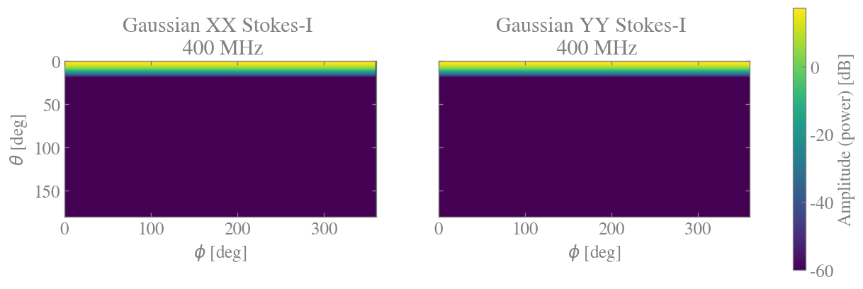
5. Directly constructing analytic power beams
TIRSPowerBeam.from_gaussian and TIRSPowerBeam.from_airy construct scalar
(typically intensity) power beam patterns directly, without going through voltage beams.
As with the voltage-beam constructors, both use a power-beam FWHM of approximately
\(1.029\,\lambda / D_\mathrm{eff}\) by default.
Key differences from the voltage-beam path:
- The pattern is a power pattern, not a field amplitude — no
sqrtis applied. The Airy pattern is \((2J_1(x)/x)^2\); the Gaussian uses exponent \(/2\) rather than \(/4\). pol_productandsky_polmust be specified manually.- This path is a simplified scalar-beam workflow and does not capture the polarisation structure that could be included when starting from voltage beams.
pbeam_gauss_xx_direct = TIRSPowerBeam.from_gaussian(
    D_eff=D_eff,
    lmax=voltage_beam_lmax,
    frequencies_MHz=frequencies_MHz,
    pol_product="XX",
    sky_pol="I",
    latitude=latitude,
    longitude=longitude,
    apply_horizon=True,
    horizon_taper_kwargs={"taper_width": np.radians(10), "apply_sqrt": False},
)
pbeam_gauss_yy_direct = TIRSPowerBeam.from_gaussian(
    D_eff=D_eff,
    lmax=voltage_beam_lmax,
    frequencies_MHz=frequencies_MHz,
    pol_product="YY",
    sky_pol="I",
    latitude=latitude,
    longitude=longitude,
    apply_horizon=True,
    horizon_taper_kwargs={"taper_width": np.radians(10), "apply_sqrt": False},
)
pbeam_airy_xx_direct = TIRSPowerBeam.from_airy(
    D_eff=D_eff,
    lmax=voltage_beam_lmax,
    frequencies_MHz=frequencies_MHz,
    pol_product="XX",
    sky_pol="I",
    latitude=latitude,
    longitude=longitude,
    apply_horizon=True,
    horizon_taper_kwargs={"taper_width": np.radians(10), "apply_sqrt": False},
)

print(
    f"Gaussian XX (direct): pol_product={pbeam_gauss_xx_direct.pol_product}, "
    f"sky_pol={pbeam_gauss_xx_direct.sky_pol}, "
    f"sht_basis={pbeam_gauss_xx_direct.sht_basis}, "
    f"alm shape={pbeam_gauss_xx_direct.alm.shape}"
)
print(
    f"Airy XX (direct):     pol_product={pbeam_airy_xx_direct.pol_product}, "
    f"alm shape={pbeam_airy_xx_direct.alm.shape}"
)
Gaussian XX (direct): pol_product=XX, sky_pol=I, sht_basis=TIRS, alm shape=(5, 201, 401)
Airy XX (direct):     pol_product=XX, alm shape=(5, 201, 401)
grid_dir = grid_template(voltage_beam_lmax)
theta_dir, phi_dir = grid_theta_phi(grid_dir, meshgrid=True)

fig, axes = plt.subplots(1, 2, figsize=(13, 5), sharey=True)

for ax, pbeam, label in zip(
    axes,
    [pbeam_gauss_xx_direct, pbeam_airy_xx_direct],
    ["Gaussian", "Airy"],
):
    pbeam_map = np.abs(pbeam.as_grid(freq_inds=0))
    pbeam_dB = 10 * np.log10(pbeam_map)
    im = ax.pcolormesh(
        np.degrees(phi_dir), np.degrees(theta_dir), pbeam_dB, vmin=-60
    )
    ax.set_title(f"{label} XX Stokes-I (direct)\n{frequencies_MHz[0]:.0f} MHz")
    ax.set_xlabel(r"$\phi$ [deg]")
    ax.set_xlim(0, 360)
    ax.set_ylim(180, 0)
    ax.set_aspect(1.0)

axes[0].set_ylabel(r"$\theta$ [deg]")
fig.colorbar(im, ax=axes, label="Power [dB]", shrink=0.8)
plt.show()

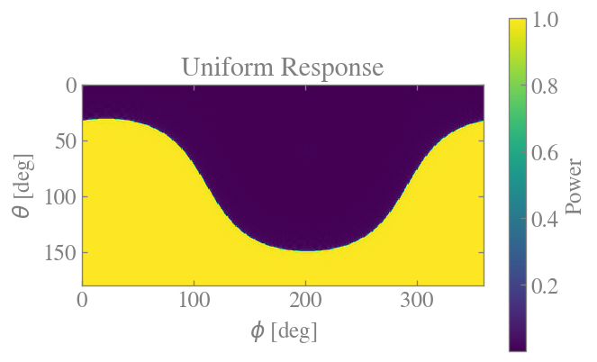
Custom patterns via from_scalar_callable
TIRSPowerBeam.from_scalar_callable accepts any function
(freq, theta, phi) -> power_map evaluated in pointing-frame coordinates,
making it straightforward to plug in arbitrary scalar beam models.
def uniform_power_pattern(freq, theta, phi):
    """Uniform primary beam response

    The callable must return shape (n_freq, nlat, nlon).  Because this pattern
    does not depend on frequency, we broadcast the spatial pattern across the
    frequency axis using freq to obtain the correct output shape.
    """
    return np.ones((freq.size,)+theta.shape)              # (n_freq, nlat, nlon)


pbeam_uniform = TIRSPowerBeam.from_scalar_callable(
    uniform_power_pattern,
    lmax=voltage_beam_lmax,
    frequencies_MHz=frequencies_MHz,
    pol_product="XX",
    sky_pol="I",
    latitude=latitude,
    longitude=longitude,
    apply_horizon=True,
)
print(f"Custom power beam alm shape: {pbeam_uniform.alm.shape}")

fig, ax = plt.subplots(figsize=(6, 5))

im = ax.pcolormesh(np.degrees(phi_dir), np.degrees(theta_dir), np.abs(pbeam_uniform.as_grid(0,0)), vmax=1)
ax.set_title(f"Uniform Response")
ax.set_xlabel(r"$\phi$ [deg]")
ax.set_xlim(0, 360)
ax.set_ylim(180, 0)
ax.set_aspect(1.0)

ax.set_ylabel(r"$\theta$ [deg]")
fig.colorbar(im, ax=ax, label="Power", shrink=0.8)
plt.show()
Custom power beam alm shape: (5, 201, 401)
pbeam_gauss_xx_direct.to_zarr_store(
    store_location=pbeam_zarr_path, group_path="gaussian_XX_I_direct"
)
pbeam_airy_xx_direct.to_zarr_store(
    store_location=pbeam_zarr_path, group_path="airy_XX_I_direct"
)
print("Saved direct power beams to Zarr store.")
Saved direct power beams to Zarr store.