Tutorial: Advanced functions
Here, we introduce some more advanced functionalities of trianglechain
import numpy as np
from trianglechain import TriangleChain
from trianglechain.params import add_derived, ensure_rec
from cosmic_toolbox.colors import set_cycle
set_cycle()
def get_samples(n_samples=100000, n_dims=3, names=None):
    covmat = np.random.normal(size=(n_dims, n_dims))
    covmat = np.dot(covmat.T, covmat)
    mean = np.random.uniform(size=(n_dims))
    samples = np.random.multivariate_normal(mean=mean, cov=covmat, size=(n_samples))
    samples = ensure_rec(samples, names)
    return samples


sample1 = get_samples(names=["a", "b", "c"])
sample2 = get_samples(names=["a", "b", "c"])
sample3 = get_samples(n_dims=4, names=["a", "b", "c", "d"])
sample4 = get_samples(names=["a", "b", "d"])
Contour plots
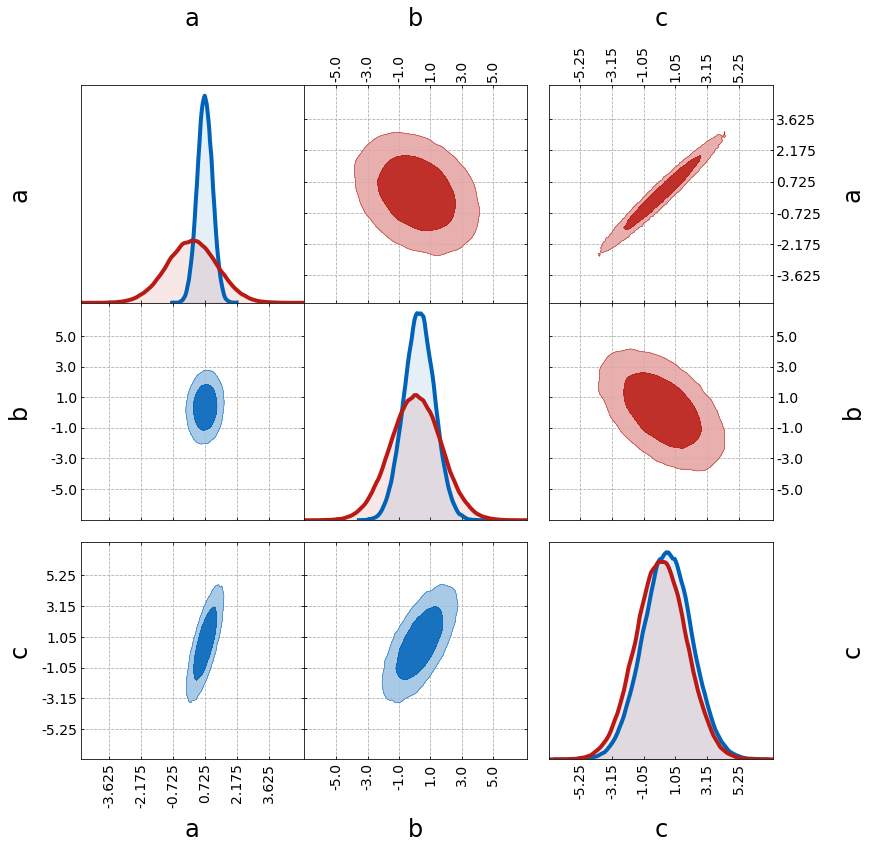
First, we show some additional plotting functionalities:
– filling the contours with fill=True
– plotting a grid with grid=True
– using the upper triangle for one of the plots with tri=upper
– grouping the parameters a & b with grouping_kwargs
– n_per_group specifies how to group the parameters
– empty_ratio determines the space between groups
– number of ticks can be varied with n_ticks
grouping_kwargs = {"n_per_group": (2, 1), "empty_ratio": 0.1}

tri = TriangleChain(fill=True, grid=True, grouping_kwargs=grouping_kwargs, n_ticks=6)
tri.contour_cl(sample1)
tri.contour_cl(sample2, tri="upper");
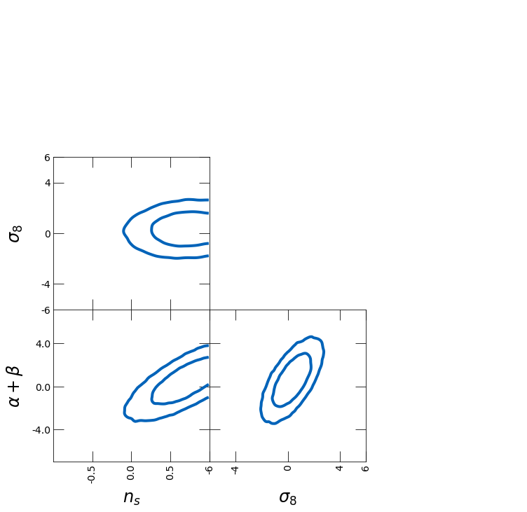
Next, we show how to change limits, ticks and labels
– limits of the plot can be changed with ranges
– ticks can be specified with ticks
– tick length can be tuned by tick_length
– 1D histograms can be turned off with plot_histograms_1D=False
– labels for the plot can be specified with labels
ranges = {"a": [-1, 1]}
ticks = {"b": [-6, -4, 0, 4, 6]}
tri = TriangleChain(
    ranges=ranges,
    ticks=ticks,
    tick_length=15,
    labels=[r"$n_s$", r"$\sigma_8$", r"$\alpha + \beta$"],
)
tri.contour_cl(sample1, plot_histograms_1D=False);
# tri.contour_cl(sample2, color=color, tri="upper");
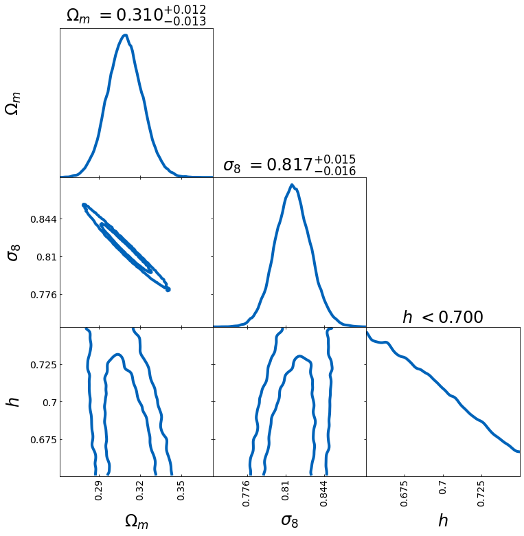
From the samples, you can directly compute the bestfit and lower and upper bounds.
– show_values=True plots the bestfit and uncertainty band for the last plotted sample
– best_fit_method specifies the way the bestfit is computed (options: mode, mean, median, best_sample (requires lnprobs))
– levels_method specifies the way the uncertainty is computed (options: hdi, percentile, PJ-HPD (requires lnprobs))
– credible_interval specifies the credible interval for the uncertainty
samples = np.load("chain.npy")
lnprobs = np.load("lnprobs.npy")

samples_c = add_derived(
    samples,
    new_param="sigma8",
    derived=samples["S8"] * np.sqrt(0.3 / samples["omega_m"]),
)
labels = [r"$\Omega_m$", r"$\sigma_8$", r"$h$"]

tri = TriangleChain(labels=labels, params=["omega_m", "sigma8", "h"])
tri.contour_cl(
    samples_c,
    show_values=True,
    levels_method="hdi",
    bestfit_method="mode",
    credible_interval=0.68,
);
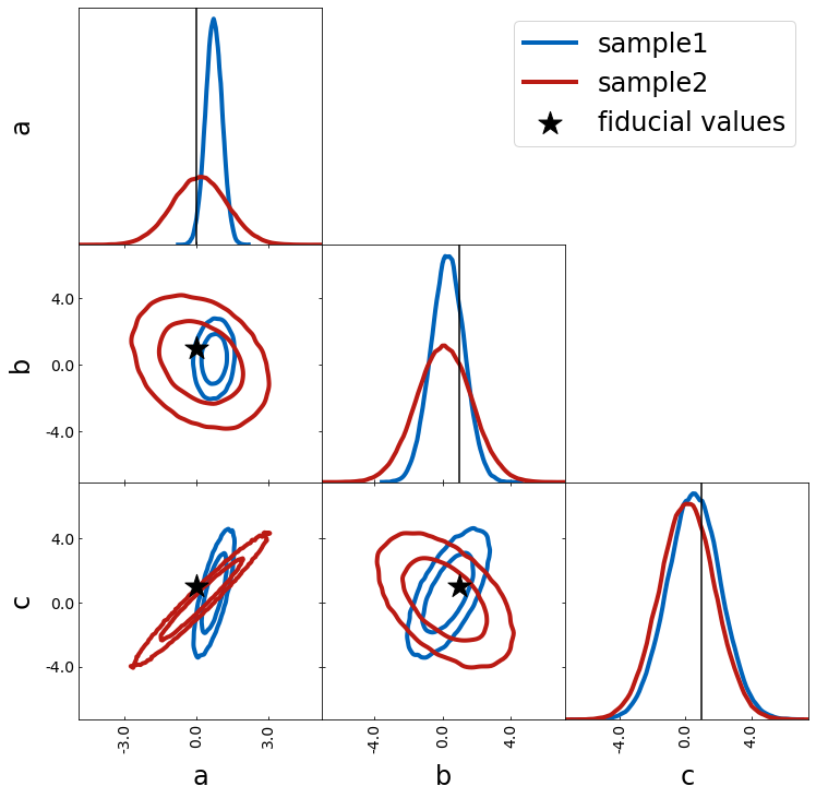
You can use scatter to show fiducal values
– combine contour_cl with scatter
– use scatter_vline_1D for the 1D projection
When combining different samples
– you can use label to label each plot
– show_legend will print the legend after this plot
fiducial = {"a": 0, "b": 1.0, "c": 1}
scatter_kwargs = {"s": 500, "marker": "*", "zorder": 299}
tri = TriangleChain(scatter_kwargs=scatter_kwargs)
tri.contour_cl(sample1, label="sample1")
tri.contour_cl(sample2, label="sample2")
tri.scatter(
    fiducial,
    label="fiducial values",
    plot_histograms_1D=False,
    color="k",
    show_legend=True,
    scatter_vline_1D=True,
);
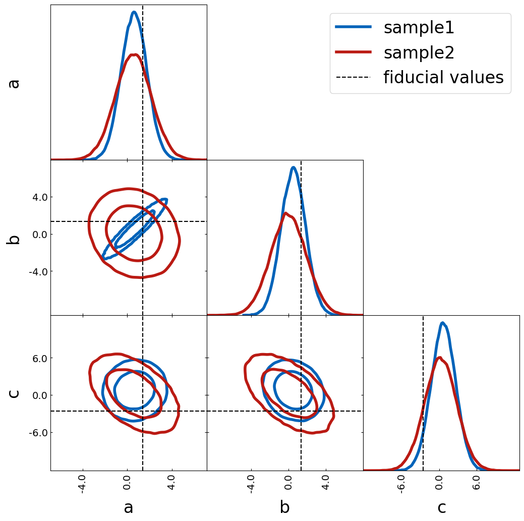
Another way how to show fiducial values is by using axlines. You can
decide if you want to show the lines in the 1D histogram by passing
plot_histograms_1D=True.
fiducial = {"a": 0, "b": 1.0, "c": 1}
tri = TriangleChain()
tri.contour_cl(sample1, label="sample1")
tri.contour_cl(sample2, label="sample2")
tri.axlines(
    sample1[:1],
    label="fiducial values",
    plot_histograms_1D=True,
    color="k",
    show_legend=True,
    axlines_kwargs={"ls": "--"},
);
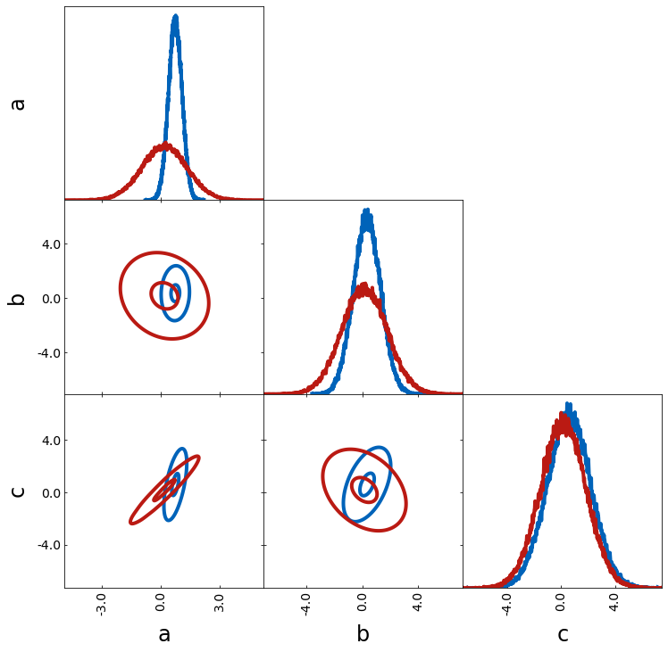
For smoothing the contours more or less, you can play around with the following
– n_bins defines the number of bins used
– density_estimation_method chooses the method used for smoothing
– de_kwargs specifies args for smoothing
de_kwargs = {
    "levels": [0.1, 0.68],
    "smoothing_parameter1D": 0.01,
    "smoothing_parameter2D": 1,
}
tri = TriangleChain(
    n_bins=1000, density_estimation_method="smoothing", de_kwargs=de_kwargs
)
tri.contour_cl(sample1, label="sample1")
tri.contour_cl(sample2, label="sample2");
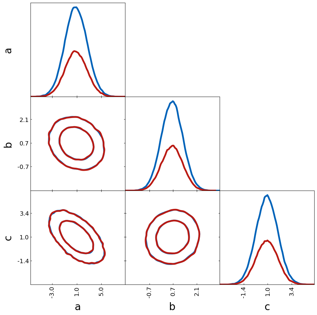
If two probability distributions are compared, it makes sense that the
1D histograms are normalized. However, one might compare two catalogs
where also the total number of objects is interesting. This can be done
by the argument histograms_1D_density=False.
tri = TriangleChain(histograms_1D_density=False)
tri.contour_cl(sample1[:100000], label="sample1")
tri.contour_cl(sample1[:50000], label="sample2");
You can combine contour plots with scatter plots to highlight
outliers—data points that fall outside the contour lines. To enable this
feature, set scatter_outliers=True. To customize the appearance of
the outlier scatter plot, use the outlier_scatter_kwargs parameter.
This accepts a dictionary of keyword arguments that are passed directly
to plt.scatter.
tri = TriangleChain()
tri.contour_cl(sample1, scatter_outliers=True);

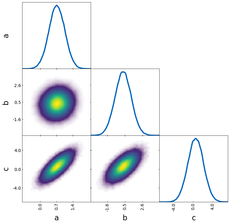
Density image
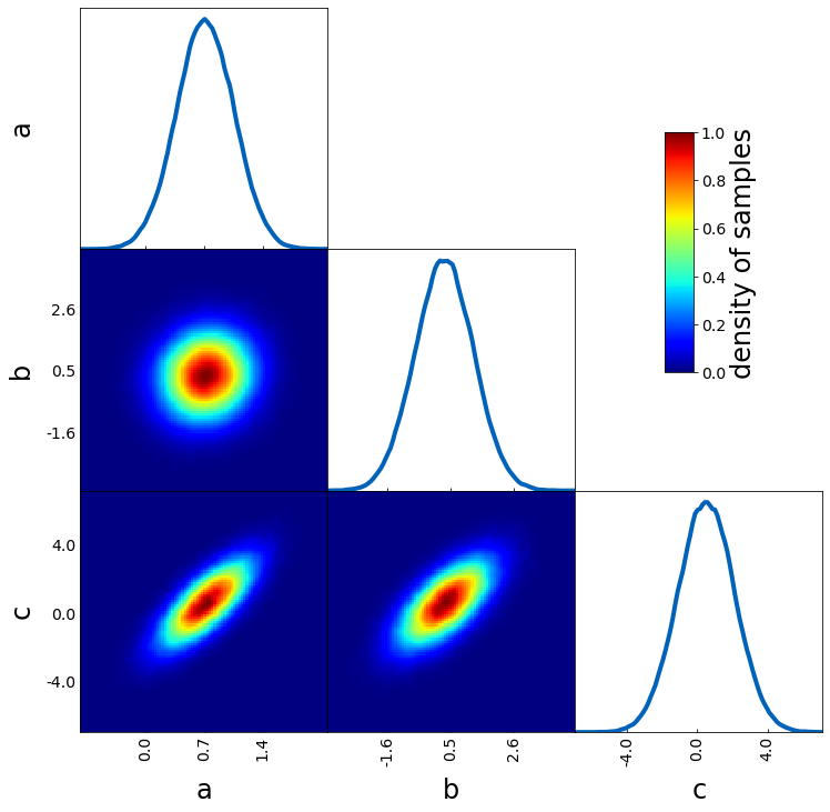
Most of the arguments introduced above can also be used for other plotting types as density images. However, there are a few specific ones for density images, e.g.
– cmap to define the colormap
– colorbar to plot a colorbar (normalized to 1)
– colorbar_label for the label of the colorbar
tri = TriangleChain()
tri.density_image(
    sample1, cmap="jet", colorbar=True, colorbar_label="density of samples"
);
If you want to have now color for the very low density areas, you can do this with
– alpha_for_low_density to turn on the fading towards transparency
–alpha_threshold to set the threshold which fraction of the maximum peak should be used for the fading
kwargs = {
    "alpha_for_low_density": True,  # set low density values to alpha
    "alpha_threshold": 0.1,
}  # how much of the cmap should be used for the transition to alpha
tri = TriangleChain(alpha_for_low_density=True, alpha_threshold=0.1)
tri.density_image(sample1);
Scatter with specified color
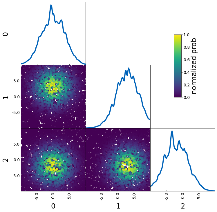
The scatter_prob plot type can be used to make a scatter plot where you specify the color.
If prob actually corresponds to a probability, you can use the default value and get the following:
samples = np.random.rand(5000, 3) * 20 - 10
sigma = 5
prob = (
    samples[:, 0] ** 2 / sigma**2
    + (samples[:, 1] - 3) ** 2 / sigma**2
    + (samples[:, 2] + 2) ** 2 / sigma**2
)
prob = np.exp(-prob)
prob /= np.sum(prob)

tri = TriangleChain(colorbar=True, colorbar_label="normalized prob")
tri.scatter_prob(samples, prob=prob);
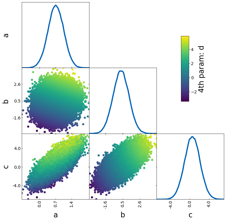
If you want to use the color to show an additional parameter (e.g. S8 when plotting sigma8 and omega_m), you have to turn off the normalization with the parameters
– normalize_prob2D=False
– normalize_prob1D=False
This way, the 1D projections still corresponds to the density of points and is not affected by prob
param4 = sample1["a"] + sample1["b"]

tri = TriangleChain(colorbar=True, colorbar_label="4th param: d")
tri.scatter_prob(sample1, prob=param4, normalize_prob2D=False, normalize_prob1D=False);
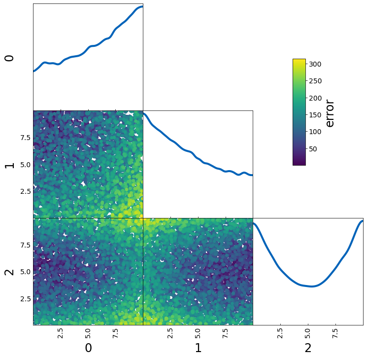
If you want to plot a specific value for the color as in the last example but the 1D projection should give you an idea where in your parameter space this value is largest, you can use
– normalize_prob2D=False
– normalize_prob1D=True (default)
This can e.g. be useful when you want to plot a fractional error across parameter space.
samples = np.random.rand(5000, 3) * 10
err = samples[:, 0] ** 2 + (10 - samples[:, 1]) ** (2) + 5 * (samples[:, 2] - 5) ** 2
tri = TriangleChain(colorbar=True, colorbar_label="error")
tri.scatter_prob(samples, prob=err, normalize_prob2D=False);
Show limits and bestfits
TriangleChain can also directly output the bestfits and limits of each parameter. The method how the limits and the bestfit is computed can be changed as well.
samples = np.load('chain.npy')
lnprobs = np.load('lnprobs.npy')

samples_c = add_derived(
    samples,
    new_param="sigma8",
    derived=samples["S8"]*np.sqrt(0.3/ samples["omega_m"])
)
labels = [r'$\Omega_m$', r'$\sigma_8$', r'$h$']
tri = TriangleChain(labels=labels, params=["omega_m", "sigma8", "h"])
tri.contour_cl(samples_c, show_values=True, levels_method="hdi", bestfit_method="mode", credible_interval=0.68);

Plain 2D Plot
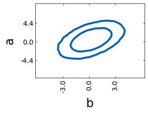
To get a plain 2D plot, the easiest is to use the LineChain module.
line = LineChain(params=["a", "b"])
line.contour_cl(sample1);
Fontsizes
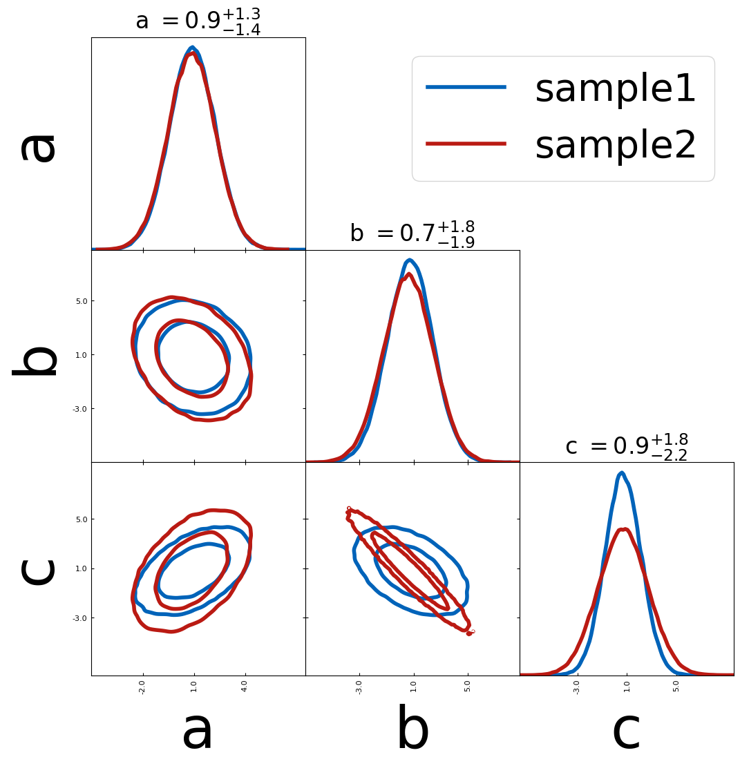
trianglechain features 4 parameters to change the fontsize without specifying any kwargs.
– label_fontsize: fontsize for the parameter
axes, is used as default for legend if legend_fontsize is not
specified.
– legend_fontsize: fontsize for the legend
– tick_fontsize: fontsize for the numbers of the ticks
– bestfit_fontsize: fontsize of the bestfit and uncertainty parameters
tri = TriangleChain(label_fontsize=60, legend_fontsize=40, tick_fontsize=8, bestfit_fontsize=24)
tri.contour_cl(sample1, label="sample1")
tri.contour_cl(sample2, label="sample2", show_legend=True, show_values=True);
and more…
For an overview of all arguments, use help(TriangleChain).
Generally, arguments passed to TriangleChain will affect all plots
whereas arguments passed to the subplots such as contour_cl will
only affect the subplot. Most arguments can be passed to both.
If you have questions, found a bug or you have suggestions for new features, feel free to contact me: silvanf@phys.ethz.ch