Tutorial: Basic plots
In this tutorial, the basic plot types of trianglechain are introduced
from trianglechain import TriangleChain, LineChain, RectangleChain
from trianglechain.TriangleChain import ensure_rec
import numpy as np
def get_samples(n_samples=100000, n_dims=3):
    covmat = np.random.normal(size=(n_dims, n_dims))
    covmat = np.dot(covmat.T, covmat)
    mean = np.random.uniform(size=(n_dims))
    samples = np.random.multivariate_normal(mean=mean, cov=covmat, size=(n_samples))
    return samples

np.random.seed(42)
samples = get_samples()
samples = ensure_rec(samples, names=["a", "b", "c"])
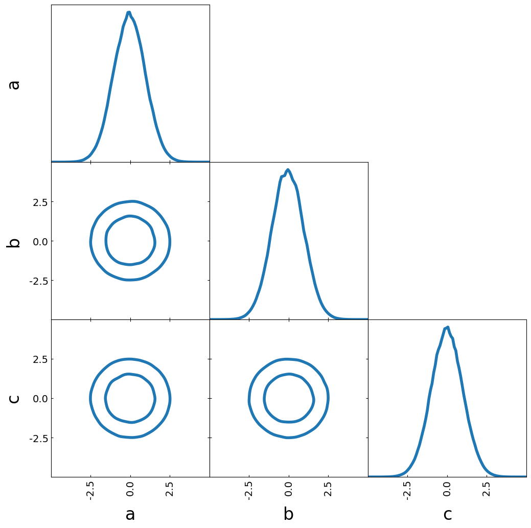
Contour plot
tri = TriangleChain()
tri.contour_cl(samples);

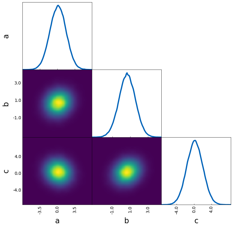
Density image
tri = TriangleChain()
tri.density_image(samples);
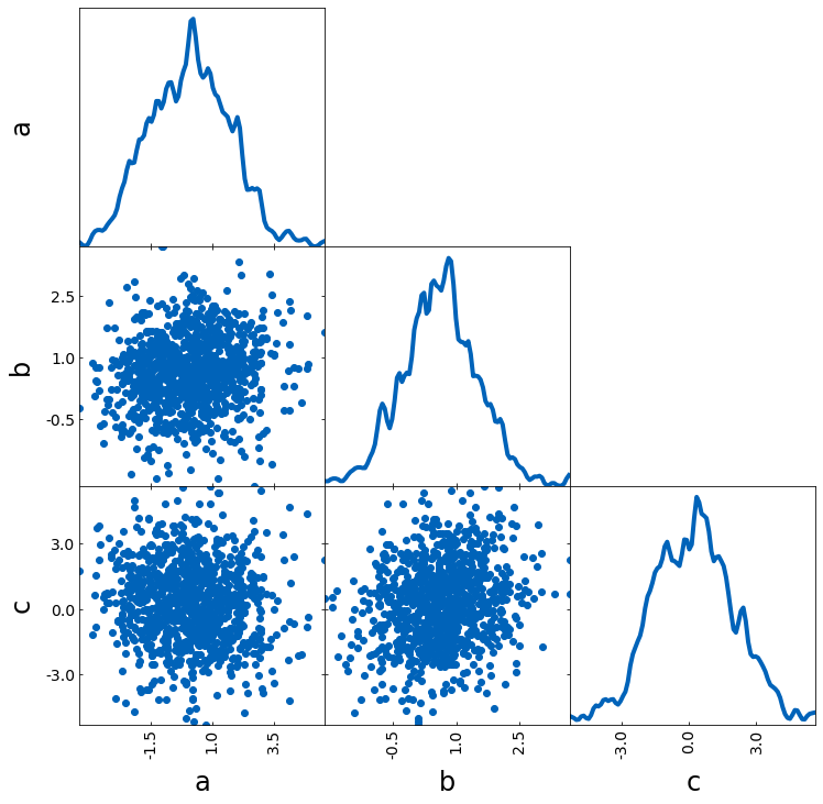
Scatter plot
tri = TriangleChain()
tri.scatter(samples[:1000]);
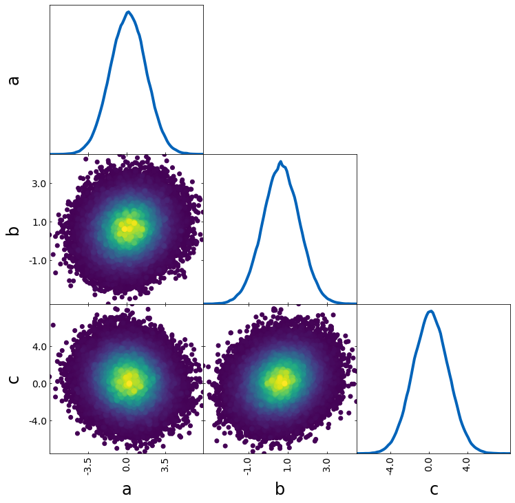
Scatter density
# scatter, color corresponds to density
tri = TriangleChain()
tri.scatter_density(samples);
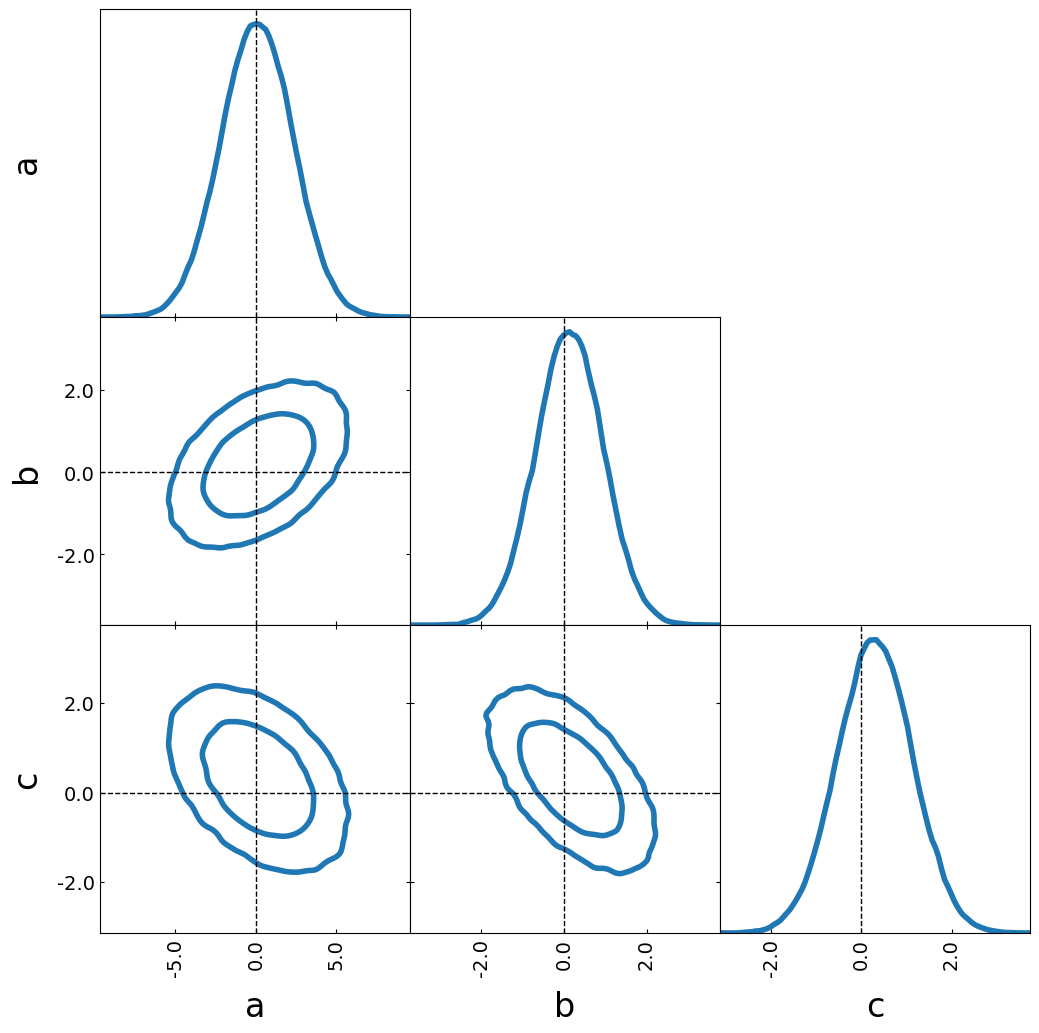
Axlines
lines = {"a": 0, "b": 0, "c": 0}

tri = TriangleChain()
tri.contour_cl(samples);
tri.axlines(lines, color="k", axlines_kwargs={"ls": "--", "lw": 1});
LineChain
All the plotting types from above can also be used in the LineChain environment. And the different plotting types can also be combined
line = LineChain()
line.contour_cl(samples);
line.density_image(samples);
line.axlines(lines, color="white");

RectangleChain
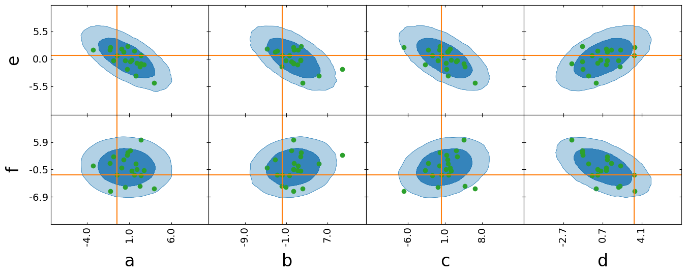
Another option is RectangleChain, here you have to define the x and y parameters
samples_rec = get_samples(n_dims=6)
samples_rec = ensure_rec(samples_rec, names=["a", "b", "c", "d", "e", "f"])
rec = RectangleChain(params_x=["a", "b", "c", "d"], params_y=["e", "f"], fill=True)
rec.contour_cl(samples_rec);
rec.axlines(samples_rec[5])
rec.scatter(samples_rec[:20]);
Samples with probability
To plot a sample where the probability of the sample is given, the
prob argument can be used (for all contour_cl, density_image
and scatter_density)
n_dims = 3
n_samples = 1000000

# Initalize grid
sample = np.random.uniform(-5, 5, size=(n_samples, n_dims))

# loglikelihood
def loglike(x, mean, covmat):
    return -0.5 * np.dot(np.dot((x - mean).T, np.linalg.inv(covmat)), (x - mean))

# Generate the covariance matrix
covmat = np.random.normal(size=(n_dims, n_dims))
covmat = np.identity(n_dims)

# Generate the mean vector
mean = np.zeros(3)

# Compute the probability for each generated sample
prob = np.zeros(n_samples)
for i in range(n_samples):
    prob[i] = loglike(sample[i], mean, covmat)

# Transform and normalize to probabilites
prob = np.exp(prob)
prob /= sum(prob)
tri = TriangleChain(names=["a", "b", "c"])
tri.contour_cl(sample, prob=prob);
