Perform source extraction

After simulating the image, it is possible to run SExtractor (Bertin & Arnouts 1996) on the image. You then receive a catalog of intrinisic and measured quantities similar to the emulator case alongside the image and the background and segmentation map by SExtractor. The same code can be run for the phenomenological and the stellar population synthesis-based versions of GalSBI by replacing Fischbacher+24 with Tortorelli+25 in the model definition.

model = GalSBI("Fischbacher+24")
model(mode="image+SE")

images = model.load_images()
image = images["image i"]
bkg = images["background i"]
seg = images["segmentation i"]

interval = PercentileInterval(95)
vmin, vmax = interval.get_limits(image)
norm = ImageNormalize(vmin=vmin, vmax=vmax)

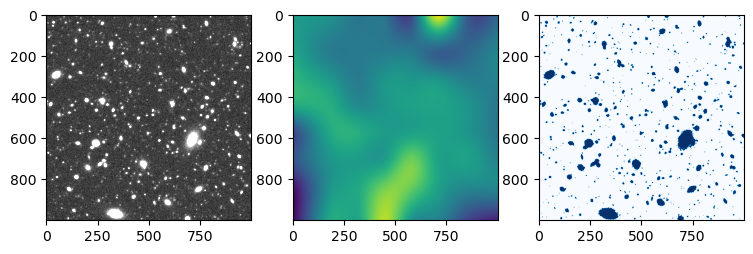
fig, axs = plt.subplots(1, 3, figsize=(9,3))
axs[0].imshow(image, cmap='gray', norm=norm)
axs[1].imshow(bkg)
axs[2].imshow(seg!=0, cmap="Blues")

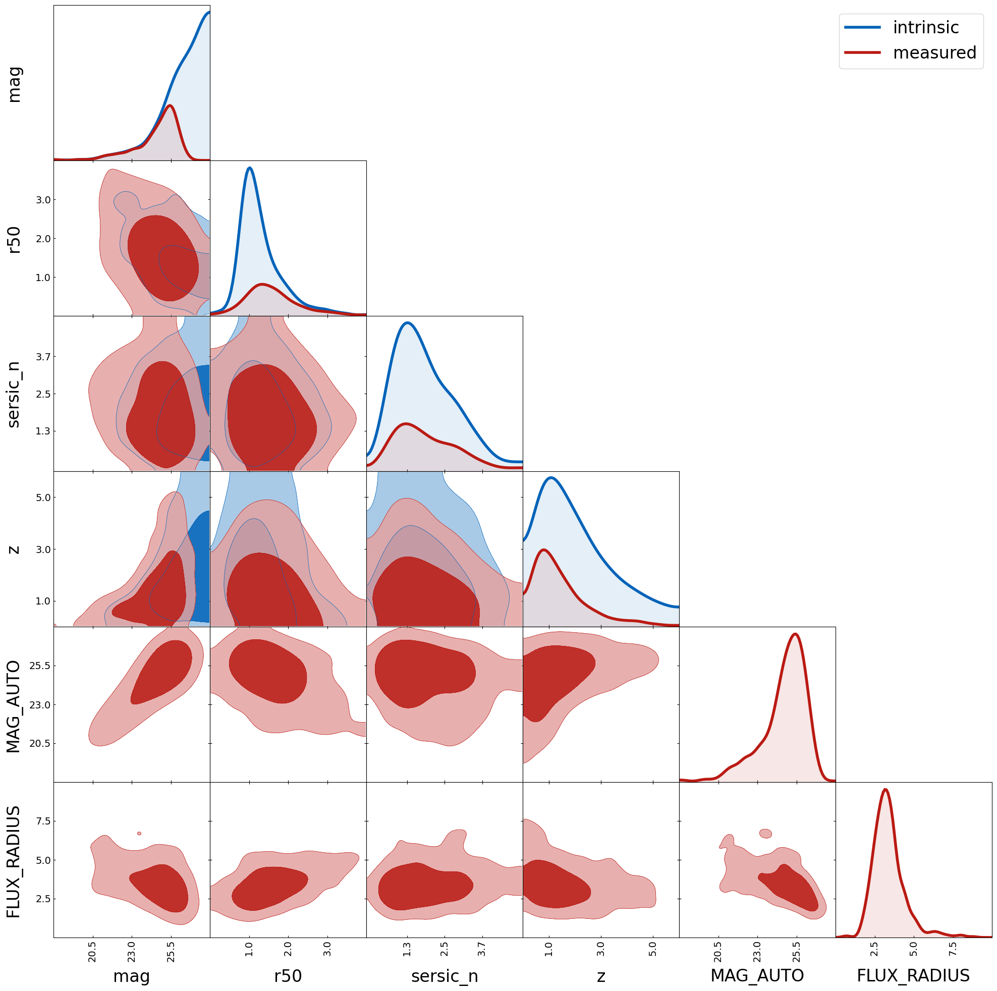
cats = model.load_catalogs()
cat_ucat = cats["ucat galaxies i"]
cat_sextractor = cats["sextractor i"]

de_kwargs = {
    "smoothing_parameter1D": 0.5,
    "smoothing_parameter2D": 0.5,
}

ranges = {
    "mag": [18, 28],
    "r50": [0, 4],
    "sersic_n": [0, 5],
    "z": [0, 6],
    "MAG_AUTO": [18, 28],
    "FLUX_RADIUS": [0, 10],
}
tri = TriangleChain(ranges=ranges, params=list(ranges.keys()), fill=True, histograms_1D_density=False, de_kwargs=de_kwargs)
tri.contour_cl(cat_ucat, label="intrinsic");
tri.contour_cl(cat_sextractor, label="measured", show_legend=True);