Saving Galaxy Spectra

By default, galaxy spectra are not saved in GalSBI, as doing so can be storage-intensive. Moreover, in the standard photometry modes, spectra are not explicitly computed. Instead, either pre-tabulated values are used to derive magnitudes from template parameters (for the phenomenological model), or magnitudes are estimated using the ProMage magnitude emulator (in the SPS model).

However, it is possible to save the Spectral Energy Distribution (SED) for each galaxy if needed. This tutorial demonstrates how to do so.

Phenomenological GalSBI

from galsbi import GalSBI
import matplotlib.pyplot as plt
import matplotlib.cm as cm
import matplotlib.colors as mcolors
import numpy as np
from scipy.integrate import trapezoid

The SED (in erg/s/cm2/Å) is saved over a rest-frame wavelength range (in Å) defined by the templates when the argument save_SEDs=True is either passed to the function or specified in the configuration file.

healpix_map = np.zeros(12 * 1024**2)
healpix_map[0] = 1

model = GalSBI("Fischbacher+24")
model(
    save_SEDs=True,
    healpix_map=healpix_map
)

The SED is saved as an HDF5 file named {file_name}_{model_index}_sed.cat. You can load it using the standard built-in loading functions. Note that the redshift of the galaxy is required to convert the SED from rest-frame to observed wavelength.

If you’re not using the combined loading mode, the SED is stored under a separate key in the returned dictionary. In combined mode, the SED is directly attached to the main catalogs — both the ucat and the SExtractor catalogs, if available.

cats = model.load_catalogs()
wavelength = cats["restframe_wavelength_in_A"]
sed_catalog = cats["sed"][1]

lamb = wavelength * (1+sed_catalog["z"])
sed = sed_catalog["sed"]

# Alternatively with combined catalogs
cats = model.load_catalogs(combine=True)
wavelength = cats["restframe_wavelength_in_A"]
total_catalog = cats["ucat galaxies"][1]

lamb = wavelength * (1+total_catalog["z"])
sed = total_catalog["sed"]

path = "../../resources/filters/"
vista_bands = ["Y", "J", "H", "Ks"]
vista_template = path + "filters_vista/Paranal_VISTA.{}_filter.dat"
sdss_bands = ["u", "g", "r", "i", "z"]
sdss_template = path + "filters_sdss/SLOAN_SDSS.{}.dat"

# Combine all filters
all_bands = sdss_bands + vista_bands
n_filters = len(all_bands)

# Generate evenly spaced rainbow colors
cmap = cm.get_cmap('rainbow', n_filters)
colors = [cmap(i) for i in range(n_filters)]
band_colors = dict(zip(all_bands, colors))  # map band name to color

# Start plotting
plt.figure(figsize=(6, 3))

# Plot SED
max_sed = np.max(sed)
plt.plot(lamb, sed, color="k", lw=0.5)

# Plot SDSS filters
for b in sdss_bands:
    lam, t = np.loadtxt(sdss_template.format(b)).T
    t /= (t.max()/max_sed)
    lambda_mean = trapezoid(lam * t, lam) / trapezoid(t, lam)
    color = band_colors[b]
    plt.fill_between(lam, t, color=color, alpha=0.2)
    plt.text(lambda_mean, 0.25*max_sed, b, color="gray", fontsize=10, ha='center', va='bottom')

# Plot VISTA filters
for b in vista_bands:
    lam, t = np.loadtxt(vista_template.format(b)).T
    t /= (t.max()/max_sed)
    lambda_mean = trapezoid(lam * t, lam) / trapezoid(t, lam)
    color = band_colors[b]
    plt.fill_between(lam, t, color=color, alpha=0.2)
    plt.text(np.mean(lam), 0.25*max_sed, b, color="gray", fontsize=10, ha='center', va='bottom')

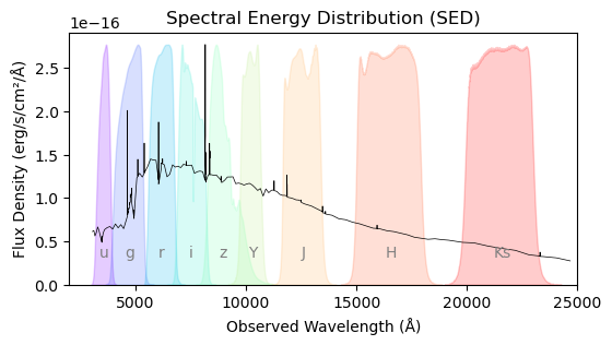
# Plot formatting
plt.xlabel("Observed Wavelength (Å)")
plt.ylabel("Flux Density (erg/s/cm²/Å)")
plt.title("Spectral Energy Distribution (SED)")
plt.ylim(bottom=0)
plt.xlim(2000, 25000)

GalSBI-SPS

When calling the Tortorelli+25 model, galaxy SEDs are computed with the SED generative package ProSpect (Robotham+20) from the physical properties drawn from GalSBI-SPS. While accessing the rest-frame wavelength array and the SEDs follows the same syntax seen above (with same units), in order to generate SEDs with GalSBI-SPS the user needs to locally install ProSpect. The pre-requisite is having R installed on your machine (https://rstudio-education.github.io/hopr/starting.html), as ProSpect is written in this programming language. We also suggest the installation of Rstudio for a more user-friendly experience.

After installing R, you can open the interpreter either by typing

R

in your bash window or using the console in Rstudio. A minimal set of steps to install ProSpect is the following:

install.packages("celestial")
install.packages("magicaxis")
install.packages("data.table")
install.packages("Rcpp")
install.packages("remotes")
remotes::install_github("asgr/Rfits")
remotes::install_github("asgr/Rwcs")
remotes::install_github("asgr/ProSpectData")
remotes::install_github("asgr/ProSpect")
install.packages("BiocManager")
BiocManager::install("rhdf5")

Further installation instructions are provided at https://github.com/asgr/ProSpect.

ProSpect combines single stellar populations (SSPs) with complex models of star-formation histories (SFHs) and other emission components (gas, dust, AGN) to generate spectral outputs for GalSBI-SPS. The original implementation of ProSpect allows the user to choose between the SSPs generated with the evolutionary SPS codes of Bruzual & Charlot (2003) and (Vazdekis et al. 2016) (EMILES). However, in Tortorelli+25 we used ProGeny to create our custom SSP. ProGeny (Robotham & Bellstedt 2025) is an SPL software package that allows for the creation of custom SSPs that can be directly input to ProSpect. In Tortorelli+25, the custom SSP follows the fiducial choices of isochrones, stellar atmospheres, and IMFs highlighted in Robotham & Bellstedt (2025); Bellstedt & Robotham (2025). This is the default SSP that galsbi calls. However, the user can supply its own SSP provided that it is in a format that ProSpect is able to read. For convenience, the user should use the ProGeny online web tool (https://progeny.datacentral.org.au/) to generate its own custom SSP as the tool output is in a format ProSpect can directly recognize.

When using the Tortorelli+25 model, the user should set both sed_generator="ProSpect" and save_SEDs=True to save galaxy SEDs. The custom SSP can then be passed to the ssp_library_filepath keyword. Leaving it at default will use the SSP in the Tortorelli+25 paper. Four additional keywords for generating SEDs with GalSBI-SPS exist. full_resolution_SEDs, which can be set to True or False, controls the output resolution of ProSpect SEDs; setting it to False coarsely resamples SSPs to a median wavelength sampling of 20 Å, which tends to speed-up the SED computation. n_cores_for_sed_generation controls the number of cores with which we parallelize the SED computation with ProSpect; this corresponds to a ~Ncores speed-up in the computation. add_AGN_component, which can be set to True or False, controls whether or not to add an AGN component emission to the galaxy SEDs. This needs to be coupled with the abs_path_temple2021 keyword that specifies the path to the qsogen folder containing the Temple+21 AGN templates. The default behaviour downloads the qsogen folder from the remote resources.

healpix_map = np.zeros(12 * 1024**2)
healpix_map[0] = 1

model = GalSBI("Tortorelli+25")
model(
    healpix_map=healpix_map
    save_SEDs=True,
    sed_generator="ProSpect",
    ssp_library_filepath=os.path.join(data_path("GalSBI_SPS_res"), "PG_Ch_Mi_C3K.fits"),
    full_resolution_SEDs=True,
    n_cores_for_sed_generation=os.cpu_count()-2,
    add_agn_component=True,
    abs_path_temple2021=os.path.join(data_path("GalSBI_SPS_res"), "qsogen")
)

Accessing the SEDs and plotting them follows the same syntax of the phenomenological model.

cats = model.load_catalogs(combine=True)
wavelength = cats["restframe_wavelength_in_A"]
total_catalog = cats["ucat galaxies"][1]

lamb = wavelength * (1+total_catalog["z"])
sed = total_catalog["sed"]

path = "../../resources/filters/"
vista_bands = ["Y", "J", "H", "Ks"]
vista_template = path + "filters_vista/Paranal_VISTA.{}_filter.dat"
sdss_bands = ["u", "g", "r", "i", "z"]
sdss_template = path + "filters_sdss/SLOAN_SDSS.{}.dat"

# Combine all filters
all_bands = sdss_bands + vista_bands
n_filters = len(all_bands)

# Generate evenly spaced rainbow colors
cmap = cm.get_cmap('rainbow', n_filters)
colors = [cmap(i) for i in range(n_filters)]
band_colors = dict(zip(all_bands, colors))  # map band name to color

# Start plotting
plt.figure(figsize=(6, 3))

# Plot SED
mask_wave = (lamb>3000)&(lamb<25000)
max_sed = np.max(sed[mask_wave])
plt.plot(lamb[mask_wave], sed[mask_wave], color="k", lw=0.5)

# Plot SDSS filters
for b in sdss_bands:
    lam, t = np.loadtxt(sdss_template.format(b)).T
    t /= (t.max()/max_sed)
    lambda_mean = trapezoid(lam * t, lam) / trapezoid(t, lam)
    color = band_colors[b]
    plt.fill_between(lam, t, color=color, alpha=0.2)
    plt.text(lambda_mean, 0.1*max_sed, b, color="gray", fontsize=10, ha='center', va='bottom')

# Plot VISTA filters
for b in vista_bands:
    lam, t = np.loadtxt(vista_template.format(b)).T
    t /= (t.max()/max_sed)
    lambda_mean = trapezoid(lam * t, lam) / trapezoid(t, lam)
    color = band_colors[b]
    plt.fill_between(lam, t, color=color, alpha=0.2)
    plt.text(np.mean(lam), 0.1*max_sed, b, color="gray", fontsize=10, ha='center', va='bottom')

# Plot formatting
plt.xlabel("Observed Wavelength (Å)")
plt.ylabel("Flux Density (erg/s/cm²/Å)")
plt.title("Spectral Energy Distribution (SED)")
plt.ylim(bottom=0)
plt.xlim(2000, 25000)